The Thirty-Third AAAI Conference on Artificial Intelligence (AAAI-19)
Using Benson’s Algorithm for Regularization Parameter Tracking
Joachim Giesen, S¨oren Laue, Andreas L¨ohne
Friedrich-Schiller-Universit¨at JenaFaculty of Mathematics and Computer Science Ernst-Abbe-Platz 2
07743 Jena, Germany
Christopher Schneider
Ernst-Abbe-Hochschule Jena Fachbereich GrundlagenwissenschaftenCarl-Zeiss-Promenade 2 07745 Jena, Germany
Abstract
Regularized loss minimization, where a statistical model is obtained from minimizing the sum of a loss function and weighted regularization terms, is still in widespread use in machine learning. The statistical performance of the result-ing models depends on the choice of weights (regulariza-tion parameters) that are typically tuned by cross-valida(regulariza-tion. For finding the best regularization parameters, the regularized minimization problem needs to be solved for the whole pa-rameter domain. A practically more feasible approach is cov-ering the parameter domain with approximate solutions of the loss minimization problem for some prescribed approxima-tion accuracy. The problem of computing such a covering is known as the approximate solution gamut problem. Existing algorithms for the solution gamut problem suffer from several problems. For instance, they require a grid on the parameter domain whose spacing is difficult to determine in practice, and they are not generic in the sense that they rely on problem specific plug-in functions. Here, we show that a well-known algorithm from vector optimization, namely the Benson al-gorithm, can be used directly for computing approximate so-lution gamuts while avoiding the problems of existing algo-rithms. Experiments for the Elastic Net on real world data sets demonstrate the effectiveness of Benson’s algorithm for regularization parameter tracking.
1
Introduction
Regularized optimization problems of the form
min
x∈Rn
`(x) +Pq
i=1αiri(x)
s.t. g(x)≤0 (P)
are still used extensively in the day-to-day practice of ma-chine learning. Here, `: Rn → R is a loss function, the
ri: Rn → R, i = 1, . . . , q are regularization terms, and theαi≥0are the correspondingregularization parameters.
Sometimes, the problem is constrained, and here the con-straints are given by a functiong:Rn→Rm.
In many machine learning applications Problem (P) is convex, i.e., all the functions`,ri, g are convex. The
op-timal solution xα of Problem (P) describes some machine
learning model, for instance the weights of a support vec-tor machine, and depends on the regularization parameters
Copyright c2019, Association for the Advancement of Artificial Intelligence (www.aaai.org). All rights reserved.
α = (α1, . . . , αq). Thus it is important to choose good
values for these parameters. The regularization parameters are typically optimized using some measure for the gener-alization error of the model on validation data, while xα
is computed from training data. Optimizing the regulariza-tion parameters is almost always a highlynon-convex prob-lem, even if Problem (P) is convex. This, essentially, leaves only searching for optimal parameters over the whole pa-rameter domain. An exhaustive search would require com-puting xα for all possible parameter values. The gamut of these solutions is called thefull solution gamut. Since it is almost never tractable to compute the full solution gamut, approximation methods and heuristics are typically used in practice. In a search heuristic, the parameter domain is sam-pled with a finite numberα1, . . . , αk of parameter vectors, an optimal solution xj, j = 1, . . . , k is computed for all
these vectors, and the best among them is chosen. A naive search approach, calledGrid Search, samples the parameter domain in a structured way on a grid. As (Bergstra and Ben-gio 2012) have pointed out, it is highly beneficial to sample the parameter domain randomly in an unstructured fashion, if the different parameter dimensions are not equally impor-tant, see Figure 1. In this case,Random Searchneeds signif-icantly fewer samples for achieving the sameapproximation error. The main disadvantage of both search approaches is
functiong
function
h
functiong
function
h
that no guarantees on the approximation error can be given, i.e., there exists nostopping rulethat determines a good grid spacing or number of random samples.
Related Work. The problem of missing approximation guarantees for the generic search methods led to a research focus on special instances of Problem (P) that we briefly review here. The special case of only one regularization term, i.e., the case q = 1, was first studied in the semi-nal work of (Efron et al. 2004) who observed that the full solution gamut of the Lasso is a piecewise linear function. The full solution gamut for problems with only one reg-ularization term, i.e., the optimal solution xα as a func-tion of the single regularizafunc-tion parameterα, is traditionally called the regularization path. In (Rosset and Zhu 2007), a fairly general theory of piecewise linear regularization paths has been developed and exact path following algo-rithms have been devised. Important special cases are sup-port vector machines whose regularization paths have been studied in (Hastie et al. 2004; Zhu et al. 2003), support vec-tor regression (Wang, Yeung, and Lochovsky 2006), and the generalized Lasso (Tibshirani and Taylor 2011). Early on it was known, see for example (Allgower and Georg 1993; Bach, Thibaux, and Jordan 2004; Hastie et al. 2004), that exact regularization path following algorithms suffer from numerical instabilities as they repeatedly need to invert a matrix whose condition number can be poor, especially when using kernels. It also turned out (G¨artner, Jaggi, and Maria 2012; Mairal and Yu 2012) that the combinatorial (and thus also computational) complexity of exact regu-larization paths can be exponential in the number of data points. These shortcomings that also show up in practice sparked interest in the development of more robust and ef-ficient approximate path algorithms (Friedman et al. 2007; Rosset 2004). By now numerically robust, approximate reg-ularization path following algorithms are known for many problems including support vector machines (Giesen, Jaggi, and Laue 2012a; Giesen et al. 2012), the Lasso (Mairal and Yu 2012), and regularized matrix factorization and comple-tion problems (Giesen, Jaggi, and Laue 2012b; Giesen et al. 2012). For a prescribed accuracyε > 0, these algorithms compute a piecewise constant approximation of the solution path, which is called anε-approximate solution gamut.
The idea of approximate solution gamuts was carried fur-ther and extended to higher dimensions, i.e.,q >1in Prob-lem (P), by (Blechschmidt, Giesen, and Laue 2015). The ba-sic algorithmic idea of this work is computing a solutionxα
to Problem (P) for some parameter vectorαand determining the region in the parameter domain, wherexαis at least an
ε-approximate solution. The algorithm then iterates over the complement of the union of the regions that are already cov-ered by someε-approximate solution. At every iteration, one element of theε-approximate solution gamut is computed. The algorithm stops once the whole parameter domain is covered. Key features of this Solution Gamut method are a well-definedstopping criterionfor a desired approxima-tion guarantee, and its efficiency that results fromadapting
to the complexity of the solution space. Fewer solutions are computed in parameter regions where the solution does not
change much. Unfortunately, the Solution Gamut method still needs a grid on the parameter domain. In contrast to Grid Search, here the grid is only used for testing whether a given solution is still anε-approximate solution at the grid point. Therefore, it is enough to compute function values at the grid points which, in general, is much cheaper than solv-ing optimization problems. For providsolv-ing the guarantee that the whole parameter domain is covered by ε-approximate solutions, the grid spacing has to be chosen carefully. In the-ory, a sufficient spacing can be derived from smoothness properties, i.e., Lipschitz constants, of Problem (P), but in practice it is non-trivial to get the grid spacing right. An-other drawback is that for checking if a solution is an ε -approximate solution, the algorithm needs to compute not only solutions to Problem (P), but also solutions to its La-grangian dual problem. Furthermore, it requires problem-specific plug-in functions.
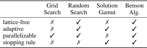
Contributions In this paper, we show that a variant of Benson’s vector optimization algorithm (Benson 1998; L¨ohne, Rudloff, and Ulus 2014) naturally allows comput-ingε-approximate solution gamuts in a way that combines the advantages of previous approaches. Benson’s algorithm comes with a clear stopping criterion and also adapts to the problem structure like the Solution Gamut method, but is grid/lattice-freein contrast to the latter. Furthermore, it works out of the box for all instances of the generic Prob-lem (P) and does not rely on probProb-lem-specific plug-in func-tions. It is easy toparallelize(B¨ucker et al. 2018) and does not need to solve dual problems. We summarize the advan-tages of Benson’s algorithm in Table 1 and compare it to the established approaches.
Table 1: Comparison of methods.
Grid Random Solution Benson Search Search Gamut Alg.
lattice-free 7 3 7 3
adaptive 7 3 3 3
parallelizable 3 3 7 3
stopping rule 7 7 3 3
2
The Solution Gamut and its Relation to
Vector Optimization
We begin by recapitulating the definition of the solution gamutfor the considered class of optimization problems and show its direct relation to thesolution conceptin the field of vector optimization
Solution Gamut. By re-scaling the objective function of Problem (P), we can assume that (P) is given as
min
x∈X fw(x) =w0`(x) +
q
X
i=1
wiri(x), (Pw)
with feasible set X = {x ∈ Rn | g(x) ≤ 0}, and regu-larization parametersw= (w0, w1, . . . , wq)∈ S ⊆Rq+1, where
S =w∈Rq+1wi≥0for alli , P q
i=0wi = 1
defines theq-dimensional standard simplex. For a given pa-rameterw∈ S, we denote byxwa global optimal solution
to Problem (Pw).
Definition 2.1. Let ε > 0 be given. We call some func-tion x¯: S → Rn an ε-approximative solution gamut of Problem (Pw), if for allw∈ S
g(¯x(w))≤0 and fw(¯x(w))−fw(xw)≤ε .
Remark2.2. Theε-approximative solution gamut in (Blech-schmidt, Giesen, and Laue 2015) is piecewise constant. Remark2.3. Forε= 0, Definition 2.1 yields the so-called
full solution gamut. Notice that the computation of full so-lution gamuts is only possible for special cases (e.g. LARS algorithm for the Lasso (Efron et al. 2004)).
Vector Optimization. For our approach, we consider the convex vector optimization problem related to (Pw), namely
min
x∈X F(x) =
h
`(x), r1(x), . . . , rq(x)
iT
w.r.t. ≤
Rq++1
(VP)
whose objective functionF:Rn → Rq+1 is vector-valued and minimized w.r.t. the component-wise partial order-ing≤
Rq++1onR
q+1:
y1≤Rq+1
+ y2 if and only if y2−y1∈R
q+1
+ ,
whereRq++1 ={y ∈Rq+1 | y
i ≥0, i = 1, . . . , q+ 1}. In
the following, the feasible setX of (VP) is assumed to be non-empty.
Connection to the Solution Gamut Problem. Our main contribution is the observation that the full solution gamut of Problem (Pw) is the set of so-calledweak minimizersof
Problem (VP).
Definition 2.4. A pointx∗ ∈ X is called aweak minimizer
of Problem (VP) if ({F(x∗)} −intR+q+1)∩F(X) = ∅,
whereF(X) ={F(x)∈Rq+1|x∈ X }is the image of the
feasible set.
The connection between the full solution gamut and the set of weak minimizers becomes intuitively clear, if one con-siders the geometry of the problems. The upper image of Problem (VP) is the set
P = closure(F(X) +Rq++1).
An optimal solution to Problem (Pw) with parametersw∈ S
is then just a weak minimizer of Problem (VP) and vice versa (see e.g., (Jahn 2011)). Let xw be an optimal
solu-tion of Problem (Pw) for parametersw∈ S, thenF(xw)is
a boundary point of the convex and closed setP and there exists a supporting hyperplane inF(xw)with normal
vec-torw(see also Figure 3 (left)). Conversely, the image of any weak minimizer of Problem (VP) is a boundary point ofP
with some normal vectorw∈ S.
Approximate Solutions. Motivated by our application in regularization parameter tracking, we are aiming at a finite representation of the full solution gamut of Problem (Pw) or,
equivalently, the set of weak minimizers of Problem (VP). Finite representations are possible for special cases, see (Hamel, L¨ohne, and Rudloff 2014), but not for a general vex vector optimization problem. Therefore, we will con-siderε-approximate solutions.
Definition 2.5. Letc∈intRq++1 be arbitrary but fixed and
assume that Problem (VP) is bounded, i.e.,P ⊆ {y}+Rq++1 holds for somey∈Rq+1. Then a nonempty, finite setX∗⊆
X is called anε-infimizerif
convF(X∗) +Rq++1−ε c⊇ P.
An ε-infimizer X∗ of (VP) is called a weak ε-solution
to (VP) if it only consists of weak minimizers.
An ε-solution X∗ provides both, an inner and an outer
polyhedral approximation of the upper imageP by finitely many minimizers. Setting Pε = convF(X∗) +Rq++1, we
have
Pε−ε c⊇ P ⊇ Pε.
Figure 2 illustrates these inclusions.
`(x)
r(x)
P
ε−
ε c
⊇ P ⊇
P
εFigure 2: Approximate Solutions.
I
0⊆ P
w
0w
1
I
0⊆ I
1⊆ P
Figure 3:Left:Initialization of Algorithm 1 with weighted-sum scalarization (Pw) forw =w0, where the dashed red line is
defined by{y|wTy=F(xw)}.Middle and right:First iteration of Algorithm 1 with regularization parameterw=w1.
3
Benson’s Algorithm
In this section, we present an algorithm for solving Prob-lem (VP), whose initial ideas go back to (Benson 1998). Since the solution gamut problem does not require the most general formulation of Problem (VP), we will adapt the ideas behind Benson’s algorithm and end up with a particu-larly simple and easy to implement variant.
Remark 3.1. Benson’s algorithm essentially exists in two variants—a primal and a dual formulation. While in the orig-inal work (Benson 1998), the primal algorithm has been derived, we will use and refine a dual scheme, whose idea goes back to (Ehrgott, L¨ohne, and Shao 2012). More details for primal and dual variants can be found, e.g., in (Hamel, L¨ohne, and Rudloff 2014) and (L¨ohne, Rudloff, and Ulus
2014).
Benson’s algorithm is especially well-suited for problems withq n, i.e., like in our context, when there are many more variables than regularization terms, because it oper-ates in the image space of the problem. The algorithm is iterative and, under the following conditions, returns a weak
ε-solution on termination—cf. (L¨ohne, Rudloff, and Ulus 2014, Theorems 4.9 and 4.14): (i) Problem (Pw) has an
op-timal solution for allw ∈ S and (ii) the feasible setX has a non-empty interior (Slater’s condition). These conditions clearly are fulfilled for the problems we consider in the fol-lowing, where all functions`,riare defined by norms
(coer-cive and continuous) andX =Rq++1.
Since for the algorithm polyhedra play a crucial role, re-member that each nonempty convex, polyhedral set A ⊆
Rq+1 either can be defined as the intersection of finitely many half-spaces, i.e.,
A=
r
\
i=1
y∈Rq+1|(wi)Ty≥bi (1)
for somer∈N,wi∈Rq+1\ {0}, andbi∈R, or by
A= conv{v1, . . . , vs}+ cone{d1, . . . , dt}, (2)
withs∈N\ {0},t ∈N, pointsvi ∈Rq+1, and directions
dj ∈
Rq+1\ {0}. We call (1) anH-representationand (2) a
V-representationofA, respectively.
The Algorithm. The now discussed (dual) variant of Ben-son’s algorithm approximates the upper imageP of Prob-lem (VP) by computing a growing sequence of inner ap-proximation polyhedraIj ={y ∈ Rq+1 | (wj)Ty ≥bj}.
After an initial inner approximationI0ofP has been
com-puted, the algorithm iteratively improves this approximation such that
I0⊆ I1⊆. . .⊆ Ij⊆. . .⊆ P.
Thereby, the algorithm relies on scalarizations of Prob-lem (VP), where the vector optimization probProb-lem is replaced by a suitable scalar optimization problem. This will be done by using the so-calledweighted-sum scalarization(Pw) (see
Section 2) with good choices for the regularization parame-terw. How thoseware chosen is described in Algorithm 1. An illustration of the initialization and the first iteration of the algorithm is given by Figure 3.
Algorithm 1Benson Algorithm
Input:Problem data (F,g), directionc, accuracyε
Output:V-rep.Ipoiand H-rep.IofPε
1: functionBENSONALGORITHM
2: T ← ∅
3: w0←( 1
q+1, . . . , 1
q+1)
T
4: x0←arg min(P
w0) 5: Ipoi← {F(x0)}
6: compute H-representationIofIpoi
7: repeat
8: choosew∈ I \T
9: xw←arg min(Pw)
10: computedc(xw)as in Equation (3)
11: ifdc(xw)> εthen
12: Ipoi← Ipoi∪ {F(xw)}
13: update the H-representationIofIpoi
14: else
15: T ←T∪ {w}
16: end if 17: untilI \T =∅
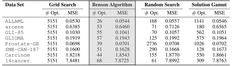
Table 2: Comparison of the minimum test MSE and number of solved optimization problems for the considered methods. Data Set Grid Search Benson Algorithm Random Search Solution Gamut
#Opt. MSE #Opt. MSE #Opt. MSE #Opt. MSE
ALLAML 5151 0.0530 26 0.0544 168 0.0557 1141 0.0546
arcene 5151 0.6385 53 0.6460 71 0.7126 180 0.6565
GLI-85 5151 0.1030 55 0.1041 70 0.1057 562 0.1051
GLIOMA 5151 0.1919 57 0.1943 125 0.1992 575 0.1964
Prostate-GE 5151 0.0698 39 0.0701 2736 0.0708 1026 0.0702
SMK-CAN-187 5151 0.1600 51 0.1628 290 0.1668 128 0.1673
Carcinom 5151 1.8218 44 1.8543 155 1.8770 550 1.8661
14cancer 5151 7.8481 68 7.8725 61 7.8992 309 7.8763
Algorithm 1 consists of two crucial phases, the initializa-tion and the main iterainitializa-tion, which we now describe in more detail.
Initialization. For computing an initial inner approxima-tionI0of the upper imageP, one can use the weighted-sum
scalarization with weightsw0= (q+11 , . . . ,q+11 )T∈Rq+1. Problem (Pw) then returns a solutionx0, whose image point
F(x0)∈ ∂P lies on the boundary of the upper image. We
set
I0={F(x0)}+Rq+1.
Figure 3 (left) illustrates this process.
Benson Iteration. At the beginning of each iteration,Ij
is given by a V-representation and has to be converted into an H-representation. This is done by facet enumeration, see (Bremner, Fukuda, and Marzetta 1998). Then, we se-lect one hyperplane{y ∈ Rq+1 | wTy = b} of the cur-rent approximationIj, represented by its normal vectorw,
and solve the scalarized problem (Pw). The distance, the
hyperplane is moved inw-direction, is justb−wTF(xw).
But since we compute anε-approximation w.r.t. the direc-tionc, we have to take the angle betweenwandc into ac-count. Therefore, the distance, the hyperplane is moved in
c-direction, is given by
dc(xw) =
cTw
kck2kwk2 b−w
TF(xw)
. (3)
Ifdc(xw) > ε, we add the optimal solutionxwof (Pw) to
our inner approximation and obtain
Ij+1= conv (Ij∪F(xw)) +Rq++1.
If otherwise dc(xw) ≤ ε, we continue with checking the
next hyperplane of the inner approximation.
Remark 3.2 (Outer Approximation). By saving the moved hyperplanes of each iteration, it would also be possible to generate an outer approximation of the upper imageP with-out further costs—cf. (L¨ohne, Rudloff, and Ulus 2014, Re-mark 4.3(2)). But since we aim for feasible solutions, this
step is omitted here.
4
Experiments
In our implementation of Algorithm 1, we used Gurobi (Gurobi Optimization 2016) for solving the scalarized problems (Pw). Facet enumeration is done by bensolve
tools(Ciripoi, L¨ohne, and Weißing 2018). We fixed the di-rection parameterc= (1, . . . ,1)T.
The Elastic Net. We apply Benson’s algorithm to the problem of linear regression, where we consider the Elastic Net regularization (Zou and Hastie 2005). The correspond-ing optimization problem reads as
min
x∈Rn 1
2kAx−bk
2
2+βkxk1+
α
2 kxk
2
2 , (EN)
whereA∈Rm×n,b∈Rm, and the regularization parame-ters areα, β∈R+. Thus, we haveq= 2.
Remark 4.1. Settingβ = 0in Problem (EN) yieldsRidge regression, whileα = 0results inLasso regression. Both scenarios haveq= 1regularization parameter and are later used to study the complexity of Benson’s algorithm.
Data Sets. A common application for the Elastic net is mi-croarray classification and gene selection(Zou and Hastie 2005, Section 6). In typical microarray data sets, there are thousands of genes but only a few samples. The Elastic Net turned out to be well-suited for such datasets since it com-bines the advantages of variable selection (L1-norm) and
grouped selection (L2-norm), especially for the m n
case.
For our experiments, we use the following data sets, which are well-known from the literature:
• ALLAMLwithm= 7,129features andn= 72instances,
• arcenewithm= 10,000andn= 200,
• GLI-85withm= 22,283andn= 85,
• GLIOMAwithm= 4,434andn= 50,
• Prostate-GEwithm= 5,966andn= 102,
• SMK-CAN-187withm= 19,993andn= 187,
• Carcinomwithm= 9,182andn= 174,
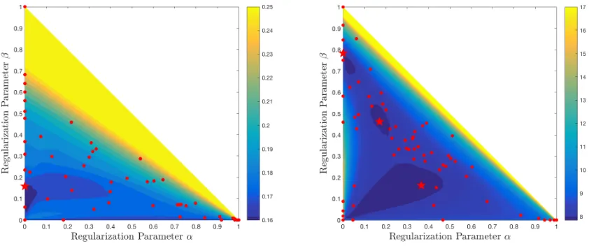
Figure 4: Shown are the test MSE values for theSMK-CAN-187(left) and 14cancer(right) data sets. The results of the fine-mesh Grid Search are depicted by colors. The iterates of Benson’s algorithm are illustrated by red points, and red stars indicate the best resp. the three best parameter combinations. All of them are located in the dark blue areas of low MSE.
Data Preparation. For all data sets,70%of the data have been used for training, and30%have been hold out for test-ing. We localize and standardize the training data, such that the response is centered and the predictors are standardized:
mtrain
X
i=1
btraini = 0,
mtrain
X
i=1
Atraini,j = 0,
mtrain
X
i=1
Atraini,j 2
= 1,
for j = 1, . . . , n. We then re-use the training parameters (mean and standard derivation) to scale the test data sets, since they should be treated as new, unseen data.
Experimental Setup. Our aim is finding regularization parametersα, βfor Problem (EN), such that its optimal so-lutionxα,β yields a low mean squared error (MSE) on the
test data set. For this purpose, we compare Benson’s algo-rithm with Grid Search, Random Search, and the Solution Gamut method of (Blechschmidt, Giesen, and Laue 2015). We proceed as follows: First, we re-scale Problem (EN) such thatα, β∈[0,1](compare Section 2),
min
x∈Rn
1−α−β
2 kAx−bk
2
2+βkxk1+
α
2 kxk
2
2. (EN
0)
Second, we compute a fine-mesh solution with Grid Search by solving (EN0) for allα, β ∈ {0,0.01,0.02, . . . ,1}. The minimum test MSE for the fine-mesh solution is used as a baseline. We then run Benson’s algorithm with approxima-tion errors ε = 0.1 (for the first six data sets) andε = 1 (for the last two data sets), resp., depending on the scale of the objective function values. After reporting the resulting minimum MSE, we run Random Search (averaged over 10 runs for each data set) and the Solution Gamut method until they reach at least the same MSE as Benson’s algorithm. We report the minimum MSE for both methods that has been obtained until this iteration.
Remark4.2. We only use the fine-mesh Grid Search for gen-erating a baseline. Coarse grids are omitted in the compar-ison, since, in general, Random Search is superior to Grid Search (cf. (Bergstra and Bengio 2012)).
Remark 4.3. Notice that Random Search and the Solution Gamut method get a big advantage by knowing the test MSE to be reached. Especially Random Search would not have a useful stopping criterion otherwise, in contrast to the Solu-tion Gamut method and Benson’s algorithm.
Results. Table 2 reports the results of our experiments. As can be seen, the minimum MSE computed by Ben-son’s algorithm reaches the fine-mesh Grid Search MSE up to0.3–2.6%(on average1.3%) by only having solved ap-prox. 1/100 of the number of optimization problems. On most examples, Random Search also performs well, but overall loses to Benson’s algorithm. The biggest limitation of Random Search is the missing stopping criterion.
It also turns out that Benson’s algorithm is the clear win-ner over the Solution Gamut method. On the average of the problem instances that we considered, Benson’s algorithm outperforms the Solution Gamut method by an order of mag-nitude in the number of optimization problems to be solved. Both approaches rely on a similar idea by exploiting the structure of the underlying optimization problem to generate good predictions. But due to the vector optimization setup, Benson’s algorithm does not need a grid for the regulariza-tion parameter space which ends up as a great benefit.
Figure 6 is an example, how Benson’s algorithm approxi-mates the upper image of the corresponding vector optimiza-tion problem. Among all vertices of the approximaoptimiza-tion, the one with the best test MSE is chosen—see Figure 4 (right).
combi-10−2 10−1 100
101
102 103
104
1/ε Elastic Net
10−2 10−1 100
101
102 103
1/√ε Lasso Regression
10−3 10−2 10−1
101
102 103
1/√ε Ridge Regression
ALLAML arcene Carcinom GLI GLIOMA Prostate-GE SMK-CAN 14cancer
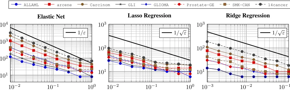
Figure 5: Log-log complexity plots of Alg. 1 for the Elastic Net (left), Lasso regression (middle) and Ridge regression (right).
600 1000 500
400 800 300 200
600 100
0 400
200 350 300 250 200 150
0 100
50 0
Figure 6: Approximation of the upper image P for the 14cancerdata set using Algorithm 1 withε= 1.
nations in “flat” areas, to obtain an overall good approxima-tion. I.e., it only generates one weight combination for the big yellow area, where the predictor is zero, because the reg-ularization terms are too dominant in Problem (EN0). Grid Search almost uses one third of its iterations to explore this area. This case is typical for most of the considered data sets.
Case Study14cancer. Figure 4 (right) shows the test MSE for the14cancerdata set. Here, we have a good ex-ample that finding the best predictor among all solutions of the regularized optimization problem is itself anon-convex
problem. There are three non-connected, dark blue areas, where certain parameter combinations(α, β)yield predic-tors with good test MSE. Benson’s algorithm computes an
ε-approximate solution for this data set in 68 iterations (red points) and thereby is able to find a representative predictor for each dark blue area (red stars). All of these three pre-dictors yield a test MSE below 7.9500, while having dif-ferent sparsity properties. From bottom to top, the three best computed predictors have 1814, 445, and 79 non-zeros, resp. Therefore, the user is able to decide between three similarly
good candidates of very different sparsity.
While this is the only example, where Random Search needed slightly less iterations than Benson’s algorithm, it was only able to find a good predictor from one of the three interesting areas.
Complexity. In (Blechschmidt, Giesen, and Laue 2015), a lower bound ofΩ(ε−q/2)for the number of optimization
problems that need to be solved for anε-approximate solu-tion gamut has been proven. For the Elastic Net (EN), we have q = 2and thus a lower bound of Ω(1/ε) of neces-sary optimization problems. In Figure 5 (left), one can see that Benson’s algorithm experimentally matches this lower bound.
Additionally, we carried out experiments for the Lasso and Ridge regression withq= 1, implying a lower bound of Ω(1/√ε). Benson’s algorithm also matches this bound—see Figure 5 (middle and right).
5
Conclusion
We have shown that Benson’s vector optimization algorithm can be used for regularization parameter tracking with pre-scribed approximation guarantees. The fairly simple algo-rithm that works out of the box and does not rely on problem specific functions combines the advantages of previously known regularization parameter tracking methods: (i) it has a well-defined stopping criterion for a prescribed approxi-mation guarantee, and (ii) it adapts to the problem structure and works grid-free, which entails fewer optimization prob-lems to be solved.
Acknowledgments
Joachim Giesen and S¨oren Laue acknowledge funding by Deutsche Forschungsgemeinschaft (DFG) under the grant GI 711/3-2. S¨oren Laue has been funded by Deutsche Forschungsgemeinschaft (DFG) under grant LA 2971/1-1. Christopher Schneider acknowledges financial support by Carl-Zeiss-Stiftung.
References
Allgower, E., and Georg, K. 1993. Continuation and path following. Acta Numerica2:1–64.
Bach, F. R.; Thibaux, R.; and Jordan, M. I. 2004. Com-puting regularization paths for learning multiple kernels. In
Advances in Neural Information Processing Systems (NIPS).
Benson, H. P. 1998. An Outer Approximation Algorithm for Generating All Efficient Extreme Points in the Outcome Set of a Multiple Objective Linear Programming Problem.
Journal of Global Optimization13(1):1–24.
Bergstra, J., and Bengio, Y. 2012. Random Search for Hyper-Parameter Optimization. Journal of Machine Learn-ing Research13(1):281–305.
Blechschmidt, K.; Giesen, J.; and Laue, S. 2015. Tracking approximate solutions of parameterized optimization prob-lems over multi-dimensional (hyper-)parameter domains. InInternational Conference on Machine Learning (ICML), 438–447.
Bremner, D.; Fukuda, K.; and Marzetta, A. 1998. Primal-Dual Methods for Vertex and Facet Enumeration. Discrete & Computational Geometry20(3):333–357.
B¨ucker, H.; L¨ohne, A.; ing, B. W.; and Zumbusch, G. 2018. On Parallelizing Benson’s Algorithm: Limits and Opportu-nities. InInternational Conference on Computational Sci-ence and Its Applications, 653–668.
Ciripoi, D.; L¨ohne, A.; and Weißing, B. 2018. Calculus of convex polyhedra and polyhedral convex functions by uti-lizing a multiple objective linear programming solver. Opti-mization.
Efron, B.; Hastie, T.; Johnstone, I.; and Tibshirani, R. 2004. Least angle regression. The Annals of Statistics32(2):407– 499.
Ehrgott, M.; L¨ohne, A.; and Shao, L. 2012. A dual variant of Benson’s “outer approximation algorithm” for multiple ob-jective linear programming.Journal of Global Optimization
52(4):757–778.
Friedman, J.; Hastie, T.; H¨ofling, H.; and Tibshirani, R. 2007. Pathwise Coordinate Optimization. The Annals of Applied Statistics1(2):302–332.
G¨artner, B.; Jaggi, M.; and Maria, C. 2012. An Exponential Lower Bound on the Complexity of Regularization Paths.
Journal of Computational Geometry (JoCG)3(1):168–195.
Giesen, J.; M¨uller, J. K.; Laue, S.; and Swiercy, S. 2012. Ap-proximating Concavely Parameterized Optimization Prob-lems. In Advances in Neural Information Processing Sys-tems (NIPS), 2114–2122.
Giesen, J.; Jaggi, M.; and Laue, S. 2012a. Approximating parameterized convex optimization problems. ACM Trans-actions on Algorithms9(1):10.
Giesen, J.; Jaggi, M.; and Laue, S. 2012b. Regularization Paths with Guarantees for Convex Semidefinite Optimiza-tion. InInternational Conference on Artificial Intelligence and Statistics (AISTATS), 432–439.
Gurobi Optimization, I. 2016. Gurobi optimizer reference manual.
Hamel, A. H.; L¨ohne, A.; and Rudloff, B. 2014. Benson type algorithms for linear vector optimization and applications.
Journal of Global Optimization59(4):811–836.
Hastie, T.; Rosset, S.; Tibshirani, R.; and Zhu, J. 2004. The Entire Regularization Path for the Support Vector Ma-chine. InAdvances in Neural Information Processing Sys-tems (NIPS).
Jahn, J. 2011. Vector Optimization: Theory, Applications, and Extensions. Springer, second edition.
L¨ohne, A.; Rudloff, B.; and Ulus, F. 2014. Primal and dual approximation algorithms for convex vector optimiza-tion problems. Journal of Global Optimization60(4):713– 736.
Mairal, J., and Yu, B. 2012. Complexity analysis of the lasso regularization path. InInternational Conference on Machine Learning (ICML).
Rosset, S., and Zhu, J. 2007. Piecewise linear regularized solution paths. The Annals of Statistics35(3):1012–1030. Rosset, S. 2004. Following curved regularized optimization solution paths. InAdvances in Neural Information Process-ing Systems (NIPS).
Tibshirani, R., and Taylor, J. 2011. The solution path of the generalized lasso.The Annals of Statistics39(3):1335–1371. Wang, G.; Yeung, D.-Y.; and Lochovsky, F. H. 2006. Two-dimensional solution path for support vector regression. InInternational Conference on Machine Learning (ICML), 993–1000.
Zhu, J.; Rosset, S.; Hastie, T.; and Tibshirani, R. 2003. 1-norm Support Vector Machines. InAdvances in Neural In-formation Processing Systems (NIPS).