The Thirty-Third AAAI Conference on Artificial Intelligence (AAAI-19)
Deep Learning for Cost-Optimal Planning: Task-Dependent Planner Selection
Silvan Sievers
University of Basel Basel, Switzerland [email protected]
Michael Katz
IBM Research Yorktown Heights, NY, USA
Shirin Sohrabi, Horst Samulowitz
IBM Research Yorktown Heights, NY, USA {ssohrab,samulowitz}@us.ibm.com
Patrick Ferber
University of Basel Basel, Switzerland [email protected]
Abstract
As classical planning is known to be computationally hard, no single planner is expected to work well across many planning domains. One solution to this problem is to use online portfo-lio planners that select a planner for a given task. These port-folios perform a classification task, a known and well-researched task in the field of machine learning. The classifi-cation is usually performed using a representation of planning tasks with a collection of hand-crafted statistical features. Re-cent techniques in machine learning that are based on auto-matic extraction of features have not been employed yet due to the lack of suitable representations of planning tasks. In this work, we alleviate this barrier. We suggest representing planning tasks by images, allowing to exploit arguably one of the most commonly used and best developed techniques in deep learning. We explore some of the questions that in-evitably rise when applying such a technique, and present various ways of building practically useful online portfolio-based planners. An evidence of the usefulness of our pro-posed technique is a planner that won the cost-optimal track of the International Planning Competition 2018.
Introduction
Domain-independent planning is known to be challenging not only due to its computational complexity (Bylander 1994), but also due to the various and very different types of domains that planners are expected to solve. Consequently, research in planning has not only focused on individual planning techniques such as the predominant planning-as-heuristic-search paradigm, but also on the question of how to combine and exploit different planning techniques for solv-ing a variety of plannsolv-ing tasks.
One such approach is to create portfolios of planners to leverage their combined strengths (Seipp et al. 2012; Vallati 2012; Cenamor, de la Rosa, and Fern´andez 2013; Seipp et al. 2015). Besides parallel portfolios that are well-suited to exploit multiple CPUs, many portfolios are sequen-tial, which means that they execute one or more planners sequentially on a given task. The decision such a portfolio has to make is which planner to run next and for how long.
Copyright © 2019, Association for the Advancement of Artificial Intelligence (www.aaai.org). All rights reserved.
While some portfolios settle on a scheduleoffline(Helmert et al. 2011; N´u˜nez, Borrajo, and Linares L´opez 2014; Seipp, Sievers, and Hutter 2014a; 2014b; 2014c), i.e., ahead of exe-cution, others try to select good plannersonlinebased on the given task (Cenamor, de la Rosa, and Fern´andez 2016; 2014; 2018). The latter is based on machine learning techniques, training a classifier on planning instances, represented as a vector of hand-crafted features. The need for extracting such features manually was alleviated in machine learning com-munity with the popularization of deep learning techniques. While there exists some work employing deep learning techniques for learning policies in probabilistic planning (Toyer et al. 2018; Issakkimuthu, Fern, and Tadepalli 2018), to the best of our knowledge, there is no published work on applying deep learning to classical planning task classi-fication. The direction, however, is most promising, as evi-denced by a sequential online planning portfolio calledDelfi forDEap Learning of PortFolIos(Katz et al. 2018). Delfi1, the winning planning system of the cost-optimal track of the International Planning Competition (IPC) 2018, represents planning tasks as images and employs image convolution for binary classification. Delfi raises several interesting ques-tions regarding both the data representation and the model selection and makes some practical decisions on how to re-solve these issues.
In this work, focusing on deep learning for planning task classification for cost-optimal planning, we elaborate on the approach and revisit the decisions made by Delfi. We start by introducing a way to represent planning tasks as images. We then explore the space of possible models that exploit image convolution for planning task classification. Specifically, we explore three questions.
The first one deals with the various levels of abstraction for planner performance data. We suggest four conceptual methods: perform regression using either the raw or normal-ized total runtime to solution, or perform classification using either a discretized set of (runtime) values or a binary value encoding whether the task was solved by that planner.
third option, we select a minimal size subset of planners that achieve the same coverage on the training data.
The third question is how to generalize to previously un-seen domains, especially with training data that is not in-dependent identically distributed. One conjecture is that for good generalization to unseen domains, the training data should also be split into training and validation sets in a sim-ilar way. We experimentally compare a random split to a ran-dom split that keeps all instances of the same ran-domain in the same set, and we also consider not splitting the data for the final model training.
As this is the first work on deep learning for planning task classification, we focus on a rather broad exploration of pos-sibilities for research in this area, thus providing both the planning and machine learning community the means for fu-ture explorations of this topic. To this end, we also conclude the paper with an extensive discussion of lessons learned and possible future research.
Background
In this section, we discuss the two planning formalisms that we base our graphical representation on: the lifted represen-tation based on thePlanning Domain Definition Language (PDDL) (McDermott 2000) and the ground finite-domain representation SAS+(B¨ackstr¨om and Nebel 1995) extended with support for action cost, conditional effects, and axioms. PDDL tasks are defined over a first-order languageLthat consists of predicates, functions, a set of natural numbers, variables, and constants. Predicates are either fluentor de-rived. Atoms and literals are defined over predicates and variables/constants as in first-order logic. They are called fluent if they only contain fluent predicates, and likewise, they are called derived if they only contain derived predi-cates. Function assignments assign a natural number from the set to function terms, which are defined over functions and variables/constants as in first-order logic. Free variables of formulas overLare also defined as in first-order logic. If a formula does not have free variables, it is calledground.
GivenL, anormalized (Helmert 2009) PDDL task is a tupleΠ = hO,A, I, Giwith the following components.O is a set ofschematic operatorso=hcost(o),pre(o),eff(o)i, wherecost(o)is a function term called thecost,pre(o)is a set of literals overL called theprecondition, andeff(o)is called theeffect. Such an operator effect is a set of univer-sally quantified effectse = ∀v1, . . . , vk : cond(e).eff(e) withvi ∈ L,cond(e)a set of literals overLcalled the
(ef-fect) condition, andeff(e)a literal over Lwithout derived predicates called theeffect.Ais a set ofschematic axioms
a=head(a)←body(a), wherehead(a)is an atom with a derived predicate called theheadandbody(a)is a set of lit-erals overLcalled thebody. Free variables inbody(a)must be free in head(a), andA must be stratifiable (Thi´ebaux, Hoffmann, and Nebel 2005). Finally, I is a set of ground fluent literals overLand consistent ground function assign-ments, called theinitial state specification, andGis a set of ground literals overL, called thegoal specification.
To define the semantics of a PDDL task, we need the notion of groundinga task. Grounding is the process that instantiates all free variables of schematic operators and
axioms in all possible ways by replacing them with con-stants. That means that each operator and axiom is replaced by a set of induced ground operators and axioms. Given a PDDL task Π as above, the induced ground task is de-fined as Π = hO,A, s0, s?i, whereO andAare obtained through grounding as just described. Astatesassigns TRUE
or FALSEto all ground fluent atoms. The corresponding de-rived state JsK extends the assignment of s to all ground atoms, evaluating ground axioms as in stratified logic pro-gramming. The initial states0 assigns TRUEto all ground
atoms inIand FALSEto all others ground fluent atoms. The goals?assigns TRUEto all positive ground literals inGand FALSEto all negative ground literals inG. A ground opera-toroisapplicableinsifJsK |=pre(o). Ground atomAis true in the successor state if it has been true insandohas no effect ϕ .¬Asuch that JsK |= ϕor ifo has an effect
ϕ . AwithJsK|=ϕ. AplanforΠis a sequence of ground operators that can be subsequently applied starting ins0and
that leads to a stateswithJsK |= s?. Its costs is the accu-mulated operator costs, where the cost values are taken from the function assignments inI.
Most modern planners reason on a ground planning task representation rather than a lifted one. Since the in-duced ground task is usually prohibitively large, these plan-ners typically apply reachability analyses to transform the ground representation into a variable-based representation such as STRIPS or SAS+. In the latter, a task Π =
hV,Vd,O,A, sd, s0, s?i has the following components. V is a set of finite-domain variables v with finite-domain dom(v).Vd⊆ Vis a subset of variables calledderived
vari-ables. Apartial statesis a partial assignment over a subset
V ⊆ V of the variables, writtenvars(s), assigning a value fromdom(v)to eachv∈vars(s), writtens[v]. Ifvars(s) =
V,sis called a state. Two partial statess, s0areconsistentif
s[v] =s0[v]for allv∈vars(s)∩vars(s0).Ois a set of
op-eratorso = hcost(o),pre(o),effs(o)iwherecost(o) ∈ R+0
is called the cost, pre(o) is a partial state called the pre-condition, and effs(o) is a set of effects. Each such ef-fect e ∈ effs(o) is a tuple e = hcond(e),var(e),val(e)i, where cond(e) is a partial state called the (effect) condi-tion, var(e) ∈ V \ Vd is called the effect variable and
val(e)∈dom(var(e))theeffect value.Ais a set of axioms
a=hpre(a),var(a),val(a)i, wherepre(a)is a partial state called the precondition,var(a) ∈ Vd is called thederived
variable andval(a) ∈ dom(var(a))the derived value.sd is a partial state defined overVd, assigning to each derived variablev ∈ Vdadefault valuesd[v] ∈ dom(v).s0 is the initial stateands?a partial state called thegoal.
The semantics of a SAS+ taskΠas above is as follows. Operatorois applicable in state sifsandpre(o)are con-sistent. Effect e ∈ effs(o) fires in s if s andcond(e) are consistent. Applyingoinsleads to the states0 that is con-sistent withsexcept for all effect variablesvar(e)of effects
classical SAS+ definition to axioms, for a states, the cor-respondingderivedstateJsKis obtained fromsby applying all axioms as in stratified logic programming. As a result, each derived variablev ∈ Vd is assigned a value, starting with the default valuessd. As for PDDL tasks, plans are se-quences of operators that lead froms0tos?and their cost is the summed operator costs.
Representing Planning Tasks
The first step towards applying existing deep learning tools to learn any model of planner performance of a domain or a task is to be able to represent the planning task in a way consumable by such tools. To come up with one such rep-resentation, in this work we follow the direction explored in the SAT and CSP communities (Loreggia et al. 2016) and represent tasks as images. In the aforementioned work the textual description of an instance was turned into a grayscale image by converting each character to a pixel. Here, we in-stead want to make use of existing graph representations of planning tasks, which we deem more natural than the tex-tual description. Such representations losslessly encode the information in the planning task and are often used for sym-metry detection. In particular, we base the images on graphs used for the computation ofstructural symmetries (Shleyf-man et al. 2015) for both ground and lifted representations (Pochter, Zohar, and Rosenschein 2011; Sievers et al. 2017). We remark that these graphs originally are defined as col-ored graphs for the purpose of excluding symmetries be-tween parts of the tasks that are colored differently. Since these colors do not add to the graphs as a structural repre-sentation of the task, we omit them here.
Problem Description Graph
Originally introduced by Pochter, Zohar, and Rosenschein (2011), theproblem description graph (PDG)is a graph that represents a SAS+task for the purpose of detecting symme-tries of the task. Shleyfman et al. (2015) later showed (in the STRIPS setting) that automorphisms of the PDG are struc-tural symmetries of the task. Below, we extend the original definition to support conditional effects and axioms.
Definition 1. LetΠ =hV,Vd,O,A, sd, s0, s?ibe aSAS+
task. The problem description graph of Π is the digraph hN, Eiwith nodes
N ={n0, n?} ∪ {nv|v∈ V} ∪Nf∪NO∪ {na |a∈ A},
whereNf ={ndv |v ∈ V, d∈ dom(v)}andNO ={no | o∈ O} ∪ {neo|o∈ O, e∈effs(o)}, and edges
E=E0∪E?∪Ev∪Ea∪Eo, where
E0={hn0, nvdi |s0[v] =d}
E?={hng, ndvi |v∈vars(s?), s?[v] =d} Ev={hnv, nvdi |d∈dom(v)}
Ea={hna, ndvi |a∈ A, v∈vars(pre(a)),pre(a)[v] =d} ∪ {hna, ndvi |a∈ A,var(a) =v, val(a) =d} Eo={hno, ndvi |o∈ O, v∈vars(pre(o)),pre(o)[v] =d}
∪ {hno, neoi |e∈effs(o)} ∪ {hnd
v, neoi | hc,·,·i ∈effs(o), v∈vars(c), c[v] =d} ∪ {hne
o, ndvi | h·, v, di ∈effs(o)}.
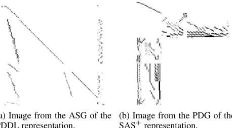
(a) Image from the ASG of the PDDL representation.
(b) Image from the PDG of the SAS+representation.
Figure 1: Lifted (left) and grounded (right) representations of task pfile01-001.pddl ofBARMAN-OPT11.
Abstract Structure Graph
Using a ground SAS+ task as a basis for the PDG means to obtain a representation that to some extent depends on the used grounding and invariant synthesis algorithms. As an alternative, we also consider theabstract structure graph (ASG)(Sievers et al. 2017) that was defined for the compu-tation of structural symmetries of PDDL tasks and used by Sievers et al. to model planning tasks as abstract structures.
Definition 2(Sievers et al., 2017). LetSbe a set of symbols, where eachs∈Sis associated with atypet(s). The set of abstract structuresoverSis inductively defined as follows:
• each symbols∈Sis an abstract structure, and
• for abstract structuresA1, . . . , An, the set{A1, . . . , An}
and the tuplehA1, . . . , Aniare abstract structures.
Using the languageLof a PDDL taskΠ, each part ofΠ can inductively be defined as an abstract structure, with the symbols ofLforming the basic abstract structures. Finally, abstract structures can be naturally turned into a graph.
Definition 3(Sievers et al., 2017, fixed). LetAbe an ab-stract structure overS. Theabstract structure graphASGA
is a digraphhN, Ei, defined as follows.
• N contains a node A for the abstract structure A. If
N contains a node for A0 = {A1, . . . , An} or A0 =
hA1, . . . , Ani, it also contains the nodes forA1, . . . , An.
• For every set (sub-)structure A0 = {A1, . . . , An} there
are edgesA0→Aifori∈ {1, . . . , n}.
• For every tuple (sub-)structure A0 = hA1, . . . , Ani, the
graph contains auxiliary nodesnA0
1 , . . . , nA
0
n , edgeA0→ n1A0 and for 1 < i ≤ n edgesniA−01 → nAi0. For each componentAi, there is an edgenA
0 i →Ai.
Converting Graphs to Images
hoc technique that colors black the left, right, up, and down neighbors of a black pixel, which helps preserving the graph structure depicted in the image when shrinking it to a fixed size. Next, we turn the image into grayscale by partitioning the image to3∗3squares and turning each square into one grayscale pixel. Finally, the size of the obtained grayscale image is resized to the constant size using antialiasing. Fig-ure 1 illustrates the different images we obtain for a task of the BARMANdomain.
We remark that our approach of turning the adjacency matrix into an image orders the graph nodes according to their type. While this is a fixed order, which we deem useful to obtain similar images for similarly structured graphs, the choice of that order may impact the resulting representation and other orders may result in images that “better” represent the planning task. Furthermore, there might also be other ways of overcoming the limitations of shrinking images to a fixed size, and more generally, constructing images from graphs. We leave exploring such alternatives as future work.
The Data
In this work we create an online portfolio for a predefined collection of planners. At runtime, we choose a planner out of that collection for a given task. This is essentially a clas-sification task for which we use the planning task represen-tation described in the previous section and image convolu-tion, one of the best performing techniques for image clas-sification. In the following, we describe the collections of planners as well as the benchmark set that we use to create data, for both training the model and testing its performance. We further discuss how to represent the performance of cost-optimal planners on the benchmarks, i.e, the total time until an optimal solution was found (or not solved). Finally, we discuss different approaches to data separation.
Component Planners
Decades of research on classical planning provide a huge pool of available planners to any portfolio method. How-ever, integrating many potentially very different planners is a technical challenge and furthermore, it is usually not easy to identify the contribution of each component to the performance of the portfolio. Therefore, for our portfolio, we picked the 17 planners from the Delfi portfolio, which Katz et al. (2018) cherry-picked from cost-optimal planners openly available prior to IPC 2018 and which they describe in detail. To evaluate our approach on a larger set of (po-tentially better) planners, we also include the other planners that participated in the latest IPC 2018 (with the exception of two planners that could not be built out of the box). These additional 12 planners are Complementary1 (Franco et al. 2018), Complementary2 (Franco, Lelis, and Barley 2018), DecStar (Gnad, Shleyfman, and Hoffmann 2018), FDMS1 and FDMS2 (Sievers 2018), Metis 2018 1 and Metis 2018 2 (Sievers and Katz 2018), Planning-PDBs (Moraru et al. 2018), Scorpion (Seipp 2018), SYMPLE 1 and SYMPLE 2 (Speck, Geißer, and Mattm¨uller 2018), and the IPC 2018 baseline, symbolic-bidirectional (Torralba et al. 2017).
Out of these planners, we consider three collections, to also test the influence of their size:CD, the collection of 17
planners from Delfi, CA, the collection of all 29 available planners, andCC, a minimal subset ofCAwhich preserves coverage of the training set. We compute CC by optimally solving the corresponding set cover problem, which results in a collection of 9 planners, 3 from Delfi (SymBA∗2014, OSS HC-PDB, DKS B-MIASMdfp) and 6 from the IPC 2018 planners (Complementary1, Complementary2, Metis2, Planning-PDBs, Scorpion, symbolic-bidirectional).
Planning Tasks
Our collection of tasks includes all benchmarks of the clas-sical tracks of all IPCs as well as some domains from the learning tracks. When domains were used in several IPCs, we only used those of the latest IPC. We further include the domainsBRIEFCASEWORLD,FERRY, andHANOI from the IPP benchmark collection (K¨ohler 1999), and the genome edit distance (GEDP) domain (Haslum 2011). We also use domains generated by the conformant-to-classical planning compilation (T0) (Palacios and Geffner 2009) and the finite-state controller synthesis compilation (FSC) (Bonet, Pala-cios, and Geffner 2009). In addition to existing tasks of these domains, we generated additional ones for some domains where generators were available. To filter out too hard tasks, we removed all tasks from the benchmark set that were not solved by any of our planners. For full details of the used benchmarks, please consult the Delfi planner abstract (Katz et al. 2018). To obtain performance data of all planners, we ran them on all planning tasks with a time bound of1800 seconds and a memory bound of7744MiB (the latter being the limit allowing to fully use all cores of our compute grid).
Planner Performance Representation
In the optimal track of the IPC, the only criterion that counts is coverage. Therefore, we need to be able to predict whether a planner from the portfolio will be able to solve the task optimally within the given time and memory bounds. The information we have, however, includes the runtime it takes a planner to solve a planning task in our training set. There are several possible ways of modeling (the final layer of) the neural network for making such a prediction.
Our first two prediction methods use regression to predict the runtime of a planner to solve a task optimally and then pick the planner with minimum runtime. The first method, calledtime, uses the raw runtime for tasks where a plan was found within the time bound of1800seconds and3600to encode that the task was not solved. The second method, callednormalized, uses the same logic but normalizes run-times to[0,1]and the additional value2. In both cases, the final layer contains a single neuron for each planner, each with a linear activation function. Its output is a real value predicting the (raw/normalized) runtime of the planner.
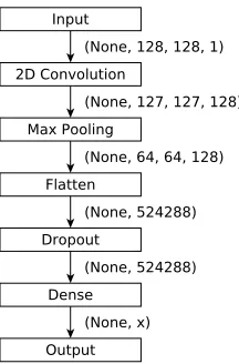
Figure 2: Graphical visualization of the CCN models. The final layer contains xneurons, which depends on the used planner collectionC: for the methodstime,normalized, and binary,x=|C|, and for the methoddiscrete,x= 4|C|.
four classes and uses a sigmoid activation function. Its out-put is a real value in[0,1]which represents the confidence that the associated discrete value is the right time interval prediction for the corresponding planner. For each planner, we compute the average over the discrete values weighted with their predicted confidence levels and choose a planner that minimizes this weighted average.
Finally, the fourth method fully abstracts away the infor-mation about the actual runtime, encoding only whether the task was solved by a planner. This corresponds to a binary classification for each planner. For this method, called bi-nary, the final layer contains a single neuron for each plan-ner, each with a sigmoid activation function. Their output is is a real value in[0,1]that represents the confidence that the planner solves the task within the time bound. We choose a planner that maximizes this value.
The rationale behind exploring different levels of abstrac-tion of the performance data is twofold. First, it might be the case that the amount of data is not sufficient to learn a meaningful model on the least abstract level. In such cases, purportedly, the more we abstract the time domain, the less data should be needed for learning. Second, it is sensible to assume that there is not much difference in terms of per-formance between planners that report solving a given task in under, say,10seconds. The actual measure might not be exact, and may vary, depending on multiple factors beyond our control. Assuming that the same logic carries over to the predicted results, choosing either of these planners should not make a big difference.
Data Separation
When learning a portfolio, the first decision one needs to make is how to separate the data into training and test sets. Since in domain-independent planning the domains are of-ten unknown a priori, we decided to use the domains from IPC 2018 as the test set. The rest of the tasks are referred as
domain-preserving split random split
CD CA CC CD CA CC
decay 0.089 0.089 0.055 4.3e-5 3.2e-5 1.5e-4
momentum 0.73 0.73 0.25 0.95 0.94 0.95
nesterov 1 1 1 1 1 1
learning rate 0.085 0.085 0.07 0.0058 0.0065 0.005
batch size 85 85 89 101 53 56
convolution filter size 3 3 5 6 2 2
dropout rate 0.48 0.48 0.39 0.49 0.49 0.5
pool filter size 3 3 2 1 1 4
Table 1: Hyper-parameters for thebinarymethod.
the training set. This separation thus recreates the scenario of the actual IPC 2018, where competitors could use all pre-viously available benchmarks for preparing their planners, and planners were then evaluated on the new benchmarks.
It is common in many learning tasks to further separate the training set, taking out a validation set. The rationale behind this is that the validation set serves as a good representation of the test set, and thus all decisions taken based on the val-idation set will hold for the test set. This, however, works under the assumption of independent identically distributed (i.i.d.) data, which breaks for planning tasks that come from various domains, and even the tasks within each domain are typically not i.i.d. Further, the domains of the IPC 2018 (our test set) were all new (in contrast to some previous IPCs that reused domains) and, to some extent, structurally very dif-ferent from old domains (in our training set). For instance, many of the tasks introduced in the IPC 2018 have actions with a much larger number of conditional effects than previ-ous tasks, which also directly impacts the PDGs/ASGs and with that, the image representations of these tasks.
Given that we want to generalize to unseen domains that are potentially different from our training data, we investi-gate the question whether a random separation of the train-ing data into traintrain-ing and validation set should keep tasks of the same domain together in one of the sets. We call the two variantsrandom splitanddomain-preserving split. One con-jecture is that domain-preserving splits should better reflect the scenario of testing on unknown, structurally different do-mains. A further interesting question to be asked is whether the validation set, and thus, any form of validation, is even needed at all, since in our case it likely does not represent the test set very accurately. We evaluate all of these options experimentally.
The data set described in this section is available online.1
Coming up with a Model
In this section, we describe how to build a model for combi-nations of prediction methods, planner sets, and data separa-tion. The training is performed on NVIDIA(R) Tesla(R) K80 GPUs. The evaluation on the test set boils down to classify-ing tasks from the test set and lookclassify-ing up the performance of the selected planner on that task. To save space, in what follows we present only the results of representing planning tasks by ASGs, i.e., using the lifted PDDL representation, which also performed better in the IPC 2018. Our
experi-1
time normalized discrete
domain-preserving split random split domain-preserving split random split domain-preserving split random split
CD CA CC CD CA CC CD CA CC CD CA CC CD CA CC CD CA CC
β1 0.975 0.99 0.98 0.96 0.96 0.89 0.89 0.6 0.67 0.99 0.77 0.91 0.99 0.93 0.99 0.99 0.98 0.98
β2 0.99 0.99 0.99 0.99 0.99 0.999 0.999 0.99 0.995 0.99 0.99 0.99 0.99 0.998 0.9995 0.99 0.99 0.9998
9.7e-9 9.9e-9 9.9e-9 4.6e-9 4.6e-9 5.1e-9 7.8e-9 5.85e-9 9.8e-9 9.99e-9 7.7e-9 9.9e-9 9.98e-9 4.5e-10 9.85e-9 9.85e-9 9.9e-9 2.5e-10
learning rate 7e-4 5e-4 6e-4 0.0049 0.0049 0.0041 0.0043 0.0049 0.0036 0.0015 5e-4 5e-4 5e-4 8e-4 5e-4 6e-4 5e-4 5e-4
batch size 124 113 53 70 70 84 85 95 89 63 58 65 94 119 114 123 77 101
convolution filter size 2 2 2 3 3 3 3 6 5 3 5 2 6 5 2 2 6 6
dropout rate 0.49 0.16 0.49 0.34 0.34 0.47 0.48 0.49 0.38 0.16 0.16 0.48 0.10 0.43 0.11 0.50 0.49 0.50
pool filter size 1 2 1 2 2 4 3 1 2 2 5 2 1 4 1 1 4 4
Table 2: Hyper-parameters for thetime,normalized, anddiscretemethods.
ments with the ground representation using PDGs showed similar behavioral trends.
Model Architecture
For our models, we employ a simple convolutional neural network (CNN) (LeCun, Bengio, and Hinton 2015) con-sisting of one convolutional layer, one pooling layer, one dropout layer, and one hidden layer. The main reason to choose a network with few parameters is to reduce the chances of overfitting given the limited amount of available data. Figure 2 shows the structure of the CNN for all predic-tion methods. The number of neurons in the last layer equals the number of planners in the chosen collection, multiplied by 4 when using the prediction methoddiscrete.
For the prediction methods time and normalized, the CNNs are trained by optimizing for mean squared error. For the other two methods, discreteandbinary, the CNNs are trained by optimizing for binary cross-entropy (Rubinstein 1997). For binary, the optimizer used is Stochastic Gradi-ent DecGradi-ent, while for the other three methods, we use the Adamoptimizer (Kingma and Ba 2015). Our tool of choice for training is Keras (Chollet 2015) with Tensorflow as a back end.
Model Selection Strategies
Although our CNNs are rather simple, they still feature a range of model hyper-parameters, which are fine-tuned em-ploying the approach by Diaz et al. (2017). Each step of the algorithm uses a 5-fold cross-validation, separating the training data into 5 subsets consisting of 20% of the data each. We optimize hyper-parameters once for each of the four prediction methods, two data separation techniques, and three planner collections, which results in24different pa-rameters settings. In order to facilitate reproducibility of our results, and to allow our methods to be transferred to other settings, Tables 1 and 2 summarize the parameters obtained for these24settings.
Experimental Evaluation
With the hyper-parameters for the 24 settings fixed, we train the models either on a subset of the training set according to the split strategy of the setting, or on the entire training data (no validation). In the former case, we train 10 models by separating the training data into 10 folds. Each fold serves once for selecting the best model trained on the remaining folds. By that, we hope to alleviate the problem of possibly
domain-preserving split random split
validation no validation validation no validation
mean std mean std mean std mean std
time
CD 50.0 4.4 57.3 1.6 57.5 1.5 57.5 0.0 CA 48.7 4.4 49.9 2.7 50.8 3.4 48.8 0.9 CC 52.6 3.9 50.5 2.2 50.7 3.9 50.3 2.3
normalized
CD 50.9 4.4 53.8 2.0 55.4 3.1 54.9 3.1 CA 51.8 3.7 50.5 2.6 48.8 1.2 49.3 1.8 CC 49.5 5.6 50.2 2.1 50.0 1.3 50.3 1.8
discrete
CD 49.5 4.0 53.7 5.9 53.9 3.3 54.1 3.0 CA 55.4 3.4 52.7 2.2 53.9 3.8 53.7 5.1 CC 50.5 1.6 51.6 3.1 58.3 5.2 53.3 1.4
binary
CD 49.6 4.0 50.2 1.4 52.0 3.3 50.3 1.1 CA 50.4 4.7 48.9 1.8 49.9 2.2 49.6 1.5 CC 53.4 3.0 49.2 2.2 52.3 2.7 51.7 3.6
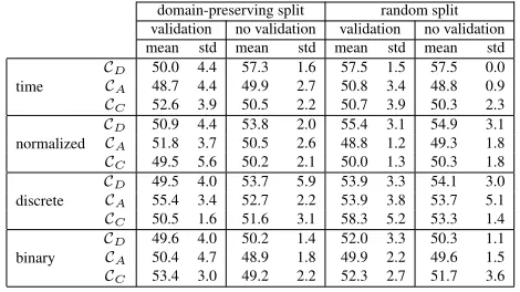
Table 3: Coverage of all 48 planners as the percentage of all 240 tasks in the test set, showing mean and standard devia-tion over the 10 models of each planner.
being (un)lucky with partitioning the training data. In the latter case, we train 10 times on the same data, taking each time the best model on that data. Thus, in both cases, we end up with 10 models for each of the48settings. We treat these as48randomized planners, run 10 times each.
Before reporting results, we briefly discuss the setting used to train Delfi. Regarding prediction, Delfi used the binary method. Regarding data separation, Delfi used a domain-preserving split (for hyper-parameter optimization) and no validation. The domain-preserving split is hand-picked, using all domains from IPCs up to 2011 as the train-ing set and those from IPC 2014 as validation set. We did not reproduce the same setting in our experiments because we considered using a hand-crafted data split to not adhere to good machine learning practice. For completeness, we still report and compare against the performance of Delfi1.
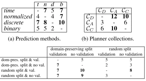
Table 3 shows coverage of all 48 planners as the percent-age of the 240 tasks of the test set (IPC 2018 domains), showing mean and standard deviation over the 10 models of each planner. In the following, we begin with comparing the different variants of our techniques against each other. To do so, we compare pair-wise each variant of the same technique, keeping everything else the same. Table 4 show matrices where each entry in row x and column y shows the number of settings where method x achieves a higher aver-age coveraver-age than method y.
t n d b time - 7 5 7 normalized 4 - 4 7 discrete 7 8 - 10 binary 5 5 2
-(a) Prediction methods.
CD CA CC
CD - 12 10
CA 3 - 6
CC 6 10
-(b) Planner collections.
domain-preserving split random split
validation no validation validation no validation
dom-pres. split & val. - 5 5 5
dom-pres. split & no val. 7 - 2 3
random split & val. 7 10 - 8
random split & no val. 7 9 3
-(c) Data split strategies with/without validation.
Table 4: Pair-wise comparison of different methods. An entry in row x and column y denotes the number of set-tings (out of 12/16/12 setset-tings for parts (a)/(b)/(c)) in which method x is better than method y. An entry is bold if x is better than y more often than vice versa.
conversely,binaryis worse than all other methods in most of the settings. However, there is no strict dominance between the methods, and the number of settings where one is better than the other is often close. Still, we think that thediscrete method might be a good way of abstracting some informa-tion on runtime of planners, while still taking it into account (in contrast tobinary).
Second, we evaluate using different planner collections (cf. Table 4b). Here, using the planners that Delfi trained on, CD, results in clearly better performance compared to using the extended planner collectionCAand the minimum set of planners to cover the training set, CC.CA andCC perform similarly to each other, withCC having a slight advantage. Clearly, our assumption that a richer set of planners, with a higher possible coverage, should result in better perfor-mance does not hold on average. It is also worth noting that the best overall performance, with a mean of58.3%, is ob-tained for a setting that uses the reduced collectionCC, how-ever with the highest standard deviation of5.2%. We think thatCA might contain too many planners for the relatively low amount of data in our training set, which resulted in models trained onCDand, to a lesser extent, onCC, making better predictions more often.
Third, we compare the two data split strategies and the op-tion to use validaop-tion or not, given a data split strategy (cf. Table 4c). We observe that using a random split with vali-dation compares favorably in most of the settings, followed by using a random split without validation, leaving random domain-preserving split strategies behind. However, there again is no strict dominance between the different strate-gies, and our conjecture that domain-preserving splits better reflect the test set does not seem to hold on average.
We now proceed with comparing our models against some baseline planners. Table 5 shows coverage, again as the per-centage of the 240 tasks of of the test set (IPC 2018 do-mains): The first three entries (two columns each) report mean and standard deviation over 1000 randomly picked planners from each collection. The next three entries show
rnd.CD rnd.CA rnd.CC oracle best
mean std mean std mean std CD CA CC C2 Sym Delfi1
42.8 8.3 45.0 8.8 50.3 9.8 67.9 72.1 70.8 58.3 57.1 60.0
Table 5: Coverage as the percentage of all 240 tasks in the test set: mean and standard deviation over 1000 randomly chosen planners of each collection; oracle coverage of each collection; three individual planners
oracle coverage of each collection. The last three entries show coverage of individual planners, namely Complemen-tary2 (C2), the best performer on the test set fromCAand
CC, Sym (SymBA∗), the best performer on the test set from
CD, and Delfi1, the winner of the cost-optimal track of IPC 2018. Note that these planners arenotthe best planners on the entire training set, where DKS-LMcut is the best plan-ner fromCD, solving 1956 out of 2530 tasks compared to SymBA* which solves 1856 tasks, and Scorpion is the best planner from CA andCC, solving 2079 out of 2530 tasks compared to Complementary2 which solves 2030 tasks.
First, comparing against the random baseline for each col-lection, we observe that our results withCDandCAstrictly dominate. However, using CC, there are 6 out of 16 set-tings where performance is worse than the random baseline. While not shown in the tables, we also verified that our mod-els are consistent w.r.t. planner selection: on average, they selected a single planner in[4.95±3.1]domains, 2 planners in[2.21±1.52]domains, 3 planners in[1.42±1.19]domains, and 4 or more planners in the remaining ~3domains.
Next, we compare against the upper end of the spectrum, namely the best planner of each collection. UsingCD, 3 out of 16 settings are better than SymBA∗, the best planner of CD, and the two best settings of these beat SymBA∗with 10 respectively 8 out of 10 models. Using the other two collec-tions, none of our settings are better than Complementary2 on average (6 out of 10 models of the best setting for CC and 3 out of 10 models of the best setting forCAbeat Com-plementary2). More generally, comparing against the per-formance of the best (oracle) planners, we see that there is still lots of room for improvement for all of the settings we tested.
Discussion and Future Work
In this work, we presented a method to apply deep learn-ing techniques to task-dependent planner selection for cost-optimal planning. For that, we introduced a principled way of representing planning tasks which is consumable by ex-isting deep learning techniques. Focusing on one such tech-nique, image convolution, we explored the space of possible ways to derive a model for classifying planning tasks. Aim-ing at presentAim-ing the reader with some of the issues that arise when the basic assumptions do not hold for existing data, we also explored various possibilities of resolving these is-sues and empirically evaluated the resulting models. Our re-sults show that there is no single recipe that works well for all tested methods. In fact, the same recipe that Delfi1 used (modulo using a different data split strategy) was found to not be the top performer among the tested methods. Further-more, also the best of our settings did not reach the actual performance of Delfi1 on average.
One likely reason is that machine learning algorithms (both for hyper-parameter optimization and network train-ing) are heavily randomized. For instance, the outcome of network training, at least in our case, depends heavily on the initial random assignment to the network variables. This re-sults in a large variance in the outcome, as verified in prelim-inary experiments aimed at retraining the model of Delfi1. Thus, further research is needed into ways of performing hyper-parameter optimization and model construction that produce a more stable outcome.
The second likely reason is the hand-crafted domain-preserving split used by Delfi1. The corresponding setting in our experiments, using a random domain-preserving split instead of the hand-crafted one, results in mean coverage significantly worse than that of Delfi1. The problem behind finding meaningful data splits in our scenario is that the most basic assumption of machine learning, which is that the data is distributed i.i.d., does not hold for planning. As a result, the common practices in machine learning may and should be questioned when applied in this setting.
One example is the way a model is selected. The common practice is to choose the model that gives the best perfor-mance on a validation set, which is separated from the train-ing set prior to the learntrain-ing phase. The assumption is that the validation set is a good representative of the test set. This as-sumption, however, does not hold in our case. To exemplify, one phenomenon that we observed when separating training data into training and validation set is that the best model chosen on the training set sometimes performed better than the one chosen on the validation set. In other words, it can be beneficial to completely ignore the data in the validation set. Consequently, more research is needed for both the question of how to split the training data of planners into a training and validation set, and for when (not) to use a validation set. In this work, we focused on generalizing to previously unseen domains, a setting used in planning competitions. In real life, however, in many cases, there is a need for solving tasks that are either new instances of existing domains or slight modifications of previously seen tasks. In such cases, some of the issues we experienced might not appear, or be-come less significant. For instance, although such data sets
are still not i.i.d., the test data would be much more simi-lar to the training data than in our setting. Furthermore, the amount of training data used in this work is relatively small by machine learning standards. Generating more data should allow using larger planning collections as components for the trained models, in turn improving the overall potential of these models.
More generally, we also see potential future work in ex-ploring alternative network architectures, leaving behind the restriction to a simplistic architecture used for image convo-lution that we used in this work. More sophisticated archi-tectures might be effective in discovering important features of planning tasks out of the task representation.
Concerning task representations, our findings clearly demonstrate that they indeed represent the tasks and that they serve well for task classification. However, our rather ad hoc approach to constructing images from graphs can certainly be improved. Furthermore, the chosen task repre-sentation is not the only possible image reprerepre-sentation for planning tasks, and image convolution is not the only tech-nique that can be applied to the chosen task representation. Exploring other task representations and other techniques to learn from these representations is a promising research di-rection.
For example, we could use the graph representation di-rectly, employing graph convolution techniques. Toyer et al. (2018) use what they call “action schema networks” for rep-resenting probabilistic planning tasks. Ma et al. (2018) use the graphs of our data set in an initial study to directly train networks on them. Alternatively, it should also be possible to learn a good representation of a planning task, which would require a way to evaluate the “quality” of a given representa-tion. We have only started exploring this direction and hope that our work will inspire other researchers to work on this problem.
Finally, since none of the ingredients of our approach is restricted to classical planning, our techniques can also di-rectly be transferred to planning settings beyond the classi-cal one, given that there exist suitable graph or image repre-sentations of non-classical tasks.
Acknowledgments
This work was supported by the European Research Council as part of the project “State Space Exploration: Principles, Algorithms and Applications” (SSX).
References
B¨ackstr¨om, C., and Nebel, B. 1995. Complexity results for SAS+planning.Computational Intelligence11(4):625– 655.
Bonet, B.; Palacios, H.; and Geffner, H. 2009. Automatic derivation of memoryless policies and finite-state controllers using classical planners. InProc. ICAPS 2009, 34–41. Bylander, T. 1994. The computational complexity of propo-sitional STRIPS planning.AIJ69(1–2):165–204.
Cenamor, I.; de la Rosa, T.; and Fern´andez, F. 2014. IBaCoP and IBaCoPB planner. InIPC-8 planner abstracts, 35–38. Cenamor, I.; de la Rosa, T.; and Fern´andez, F. 2016. The IBaCoP planning system: Instance-based configured portfo-lios. JAIR56:657–691.
Cenamor, I.; de la Rosa, T.; and Fern´andez, F. 2018. IBaCoP-2018 and IBaCoP2-2018. In IPC-9 planner ab-stracts, 9–10.
Chollet, F. 2015. https://keras.io.
Diaz, G. I.; Fokoue-Nkoutche, A.; Nannicini, G.; and Samu-lowitz, H. 2017. An effective algorithm for hyperparameter optimization of neural networks. IBM Journal of Research and Development61(4).
Franco, S.; Lelis, L. H. S.; Barley, M.; Edelkamp, S.; Mar-tines, M.; and Moraru, I. 2018. The Complementary1 plan-ner in the IPC 2018. InIPC-9 planner abstracts, 28–31. Franco, S.; Lelis, L. H. S.; and Barley, M. 2018. The Com-plementary2 planner in the IPC 2018. InIPC-9 planner ab-stracts, 32–36.
Gnad, D.; Shleyfman, A.; and Hoffmann, J. 2018. Decstar – STAR-topology DECoupled Search at its best. InIPC-9 planner abstracts, 42–46.
Haslum, P. 2011. Computing genome edit distances using domain-independent planning. InICAPS 2011 Scheduling and Planning Applications woRKshop, 45–51.
Helmert, M.; R¨oger, G.; Seipp, J.; Karpas, E.; Hoffmann, J.; Keyder, E.; Nissim, R.; Richter, S.; and Westphal, M. 2011. Fast Downward Stone Soup. InIPC 2011 planner abstracts, 38–45.
Helmert, M. 2009. Concise finite-domain representations for PDDL planning tasks.AIJ173:503–535.
Issakkimuthu, M.; Fern, A.; and Tadepalli, P. 2018. Training deep reactive policies for probabilistic planning problems. InProc. ICAPS 2018, 422–430.
Katz, M.; Sohrabi, S.; Samulowitz, H.; and Sievers, S. 2018. Delfi: Online planner selection for cost-optimal planning. In IPC-9 planner abstracts, 57–64.
Kingma, D. P., and Ba, J. 2015. Adam: A method for stochastic optimization. InProc. ICLR 2015.
K¨ohler, J. 1999. Handling of conditional effects and neg-ative goals in IPP. Technical Report 128, University of Freiburg, Department of Computer Science.
LeCun, Y.; Bengio, Y.; and Hinton, G. 2015. Deep learning. Nature521(7553):436–444.
Loreggia, A.; Malitsky, Y.; Samulowitz, H.; and Saraswat, V. A. 2016. Deep learning for algorithm portfolios. InProc. AAAI 2016, 1280–1286.
Ma, T.; Ferber, P.; Huo, S.; Chen, J.; and Katz, M. 2018. Adaptive planner scheduling with graph neural networks. arXiv:1811.00210v2 [cs.AI].
McDermott, D. 2000. The 1998 AI Planning Systems com-petition. AI Magazine21(2):35–55.
Moraru, I.; Edelkamp, S.; Martinez, M.; and Franco, S. 2018. Planning-PDBs planner. InIPC-9 planner abstracts, 69–73.
N´u˜nez, S.; Borrajo, D.; and Linares L´opez, C. 2014. Miplan and dpmplan. InIPC-8 planner abstracts.
Palacios, H., and Geffner, H. 2009. Compiling uncertainty away in conformant planning problems with bounded width. JAIR35:623–675.
Pochter, N.; Zohar, A.; and Rosenschein, J. S. 2011. Exploit-ing problem symmetries in state-based planners. In Proc. AAAI 2011, 1004–1009.
Rubinstein, R. Y. 1997. Optimization of computer simula-tion models with rare events. European Journal of Opera-tional Research99(1):89–112.
Seipp, J.; Braun, M.; Garimort, J.; and Helmert, M. 2012. Learning portfolios of automatically tuned planners. In Proc. ICAPS 2012, 368–372.
Seipp, J.; Sievers, S.; Helmert, M.; and Hutter, F. 2015. Au-tomatic configuration of sequential planning portfolios. In Proc. AAAI 2015, 3364–3370.
Seipp, J.; Sievers, S.; and Hutter, F. 2014a. Fast Downward Cedalion. InIPC-8 planner abstracts, 17–27.
Seipp, J.; Sievers, S.; and Hutter, F. 2014b. Fast Downward Cedalion. InIPC-8 Planning and Learning Part: planner abstracts.
Seipp, J.; Sievers, S.; and Hutter, F. 2014c. Fast Downward SMAC. InIPC-8 Planning and Learning Part: planner ab-stracts.
Seipp, J. 2018. Fast Downward Scorpion. InIPC-9 planner abstracts, 77–79.
Shleyfman, A.; Katz, M.; Helmert, M.; Sievers, S.; and Wehrle, M. 2015. Heuristics and symmetries in classical planning. InProc. AAAI 2015, 3371–3377.
Sievers, S., and Katz, M. 2018. Metis 2018. InIPC-9 plan-ner abstracts, 83–84.
Sievers, S.; R¨oger, G.; Wehrle, M.; and Katz, M. 2017. Structural symmetries of the lifted representation of classi-cal planning tasks. InICAPS 2017 Workshop on Heuristics and Search for Domain-independent Planning, 67–74. Sievers, S. 2018. Fast Downward merge-and-shrink. In IPC-9 planner abstracts, 85–90.
Speck, D.; Geißer, F.; and Mattm¨uller, R. 2018. SYMPLE: Symbolic Planning based on EVMDDs. InIPC-9 planner abstracts, 91–94.
Thi´ebaux, S.; Hoffmann, J.; and Nebel, B. 2005. In defense of PDDL axioms.AIJ168(1–2):38–69.
Torralba, ´A.; Alc´azar, V.; Kissmann, P.; and Edelkamp, S. 2017. Efficient symbolic search for cost-optimal planning. AIJ242:52–79.
Toyer, S.; Trevizan, F.; Thi´ebaux, S.; and Xie, L. 2018. Ac-tion schema networks: Generalised policies with deep learn-ing. InProc. AAAI 2018, 6294–6301.