The Thirty-Third AAAI Conference on Artificial Intelligence (AAAI-19)
Large-Scale Visual Relationship Understanding
Ji Zhang,
1,2Yannis Kalantidis,
1Marcus Rohrbach,
1Manohar Paluri,
1Ahmed Elgammal,
2Mohamed Elhoseiny
11Facebook Research
2Department of Computer Science, Rutgers University
Abstract
Large scale visual understanding is challenging, as it requires a model to handle the widely-spread and imbalanced distri-bution ofhsubject, relation, objectitriples. In real-world sce-narios with large numbers of objects and relations, some are seen very commonly while others are barely seen. We develop a new relationship detection model that embeds objects and relations into two vector spaces where both discriminative ca-pability and semantic affinity are preserved. We learn a visual and a semantic module that map features from the two modal-ities into a shared space, where matched pairs of features have to discriminate against those unmatched, but also maintain close distances to semantically similar ones. Benefiting from that, our model can achieve superior performance even when the visual entity categories scale up to more than 80,000, with extremely skewed class distribution. We demonstrate the efficacy of our model on a large and imbalanced benchmark based of Visual Genome that comprises53,000+objects and 29,000+ relations, a scale at which no previous work has been evaluated at. We show superiority of our model over competitive baselines on the original Visual Genome dataset with80,000+categories. We also show state-of-the-art per-formance on the VRD dataset and the scene graph dataset which is a subset of Visual Genome with200categories.
Introduction
Scale matters. In the real world, people tend to describe vi-sual entities with open vocabulary, e.g., the raw ImageNet (Deng et al., 2009) dataset has 21,841 synsets that cover a vast range of objects. The number of entities is signif-icantly larger for relationships since the combinations of
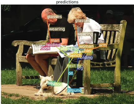
hsubject, relation, objectiare orders of magnitude more than objects (Lu et al., 2016; Plummer et al., 2017; Zhang et al., 2017c). Moreover, the long-tailed distribution of objects can be an obstacle for a model to learn all classes sufficiently well, and such challenge is exacerbated in relationship de-tection because either the subject, the object, or the relation could be infrequent, or their triple might be jointly infre-quent. Figure 1 shows an example from the Visual Genome dataset, which contains commonly seen relationship (e.g.,
hman,wearing,glassesi) along with uncommon ones (e.g.,
hdog,next to,womani).
Copyright c2019, Association for the Advancement of Artificial Intelligence (www.aaai.org). All rights reserved.
Figure 1: Relationships predicted by our approach on an im-age. Different relationships are colored differently with a re-lation line connecting each subject and object. Our model is able to recognize relationships composed of over53,000 object categories and over29,000relation categories.
Another challenge is that object categories are often se-mantically associated (Deng et al., 2009; Krishna et al., 2017; Deng et al., 2014), and such connections could be more subtle for relationships since they are conditioned on the contexts. For example, an image ofhperson,ride,horsei
could look like one ofhperson,ride,elephantisince they both belong to the kind of relationships where a person is riding an animal, buthperson,ride,horseiwould look very different from hperson,walk with,horsei even though they have the same subject and object. It is critical for a model to be able to leverage such conditional connections.
Related Work
Visual Relationship DetectionA large number of visual re-lationship detection approaches have emerged during the last couple of years. Almost all of them are based on a small vo-cabulary, e.g., 100 object and 70 relation categories from the VRD dataset (Lu et al., 2016), or a subset of VG with the most frequent object and relation categories (Zhang et al., 2017a; Xu et al., 2017).
In one of the earliest works, Lu et al. (2016) utilize the object detection output of an an R-CNN detector and lever-age langulever-age priors from semantic word embeddings to fine-tune the likelihood of a predicted relationship. Very recently, Zhuang et al. (2017) use language representations of the sub-ject and obsub-ject as “context” to derive a better classification result for the relation. However, similar to Lu et al. (2016) their language representations are pre-trained. Unlike these approach, we fine-tune subject and object representations jointlyand employ the interaction between branches also at an earlier stage before classification.
In Yu et al. (2017), the authors employ knowledge dis-tillation from a large Wikipedia-based corpus and get state-of-the-art results for the VRD (Lu et al., 2016) dataset. In ViP-CNN (Li et al., 2017), the authors pose the problem as a classification task on limited classes and therefore can-not scale to the open-vocabulary scenarios. In our model we exploit co-occurrences at the relationship level to model such knowledge. Our approach directly targets the large cat-egory scale and is able to utilize semantic associations to compensate for infrequent classes, while at the same time achieves competitive performance in the smaller and con-strained VRD (Lu et al., 2016) dataset.
Very recent approaches like Zhao et al. (2017); Plummer et al. (2017) target open-vocabulary for scene parsing and visual relationship detection, respectively. In Plummer et al. (2017), the related work closest to ours, the authors learn a CCA model on top of different combinations of the subject, object and union regions and train a Rank SVM. They how-ever consider each relationship triplet as a class and learn it as a whole entity, thus cannot scale to our setting. Our ap-proach embeds the three components of a relationship sep-arately to the independent semantic spaces for object and relation, but implicitly learns connections between them via visual feature fusion and semantic meaning preservation in the embedding space.
Semantically Guided Visual Recognition. Another par-allel category of vision and language tasks is known as zero-shot/few-shot, where class imbalance is a primary as-sumption. In Frome et al. (2013), Norouzi et al. (2014) and Socher et al. (2013), word embedding language models (e.g., Mikolov et al. (2013)) were adopted to represent class names as vectors and hence allow zero-shot recognition. For fine-grained objects like birds and flowers, several works adopted Wikipedia Articles to guide zero-shot/few-shot recognition (Elhoseiny, Saleh, and Elgammal, 2013; Elhoseiny, Elgam-mal, and Saleh, 2017; Lei Ba et al., 2015; Elhoseiny et al., 2017). However, for relations and actions, these methods are not designed with the capability of locating the objects or interacting objects for visual relations. Several approaches have been proposed to model the visual-semantic
embed-ding in the context of the image-sentence similarity task (e.g., Kiros, Salakhutdinov, and Zemel (2014); Vendrov et al. (2015); Faghri et al. (2018); Wang, Li, and Lazebnik (2016); Gong et al. (2014)). Most of them focused on lean-ing semantic connections between the two modalities, which we not only aim to achieve, but with a manner that does not sacrifice discriminative capability since our task is detection instead of similarity-based retrieval. In contrast, visual re-lationship also has a structure ofhsubject, relation, objecti
and we show in our results that proper design of a visual-semantic embedding architecture and loss is critical for good performance.
Note: in this paper we use “relation” to refer to what is also known as ‘predicate” in previous works, and “relation-ship” or “relationship triplet” to refer to ahsubject, relation, objectituple.
Method
Figure 2 shows the work flow of our model. We take an image as input to the visual module and output three vi-sual embeddings xs, xp, and xo for subject, relation, and
object. During training we take word vectors of subject, re-lation, object as input to the semantic module and output three semantic embeddingsys, yp, yo. We minimize the loss by matching the visual and semantic embeddings using our designed losses. During testing we feed word vectors of all objects and relations and use nearest neighbor searching to predict relationship labels. The following sections describe our model in details.
Visual Module
The design logic of our visual module is that a relation ex-ists when its subject and object exist, but not vice versa. Namely, relation recognition is conditioned on subject and object, but object recognition is independent from relations. The main reason is that we want to learn embeddings for subject and object in a separate semantic space from the re-lation space. That is, we want to learn a mapping from visual feature space (which is shared among subject/object and re-lation) to the two separate semantic embedding spaces (for objects and relations). Therefore, involving relation features for subject/object embeddings would have the risk of en-tangling the two spaces. Following this logic, as shown in Figure 2 an image is fed into a CNN (conv1 1toconv5 3 of VGG16) to get a global feature map of the image, then the subject, relation and object featureszs,zp,zoare
ROI-pooled with the corresponding regionsRS,RP,RO, each branch followed by two fully connected layers which out-put three intermediate hidden features hs2,hp2,ho2. For the subject/object branch, we add another fully connected layer
ws3to get the visual embeddingxs, and similarly for the ob-ject branch to getxo. For the relation branch, we apply a
two-level feature fusion: we first concatenate the three hid-den featureshs
2,h
p
2,ho2and feed it to a fully connected layer
wp3to get a higher-level hidden featurehp3, then we concate-nate the subject and object embeddingsxs andxowithhp3
CNN
conv1_1 ~ conv5_3
woman
hold
umbrella
+
+
+
+
+
+
+
+
Figure 2: (a) Overview of the proposed approach.Ls,Lp,Loare the losses of subject, relation and object. Orange, purple and
blue colors represent subject, relation, object, respectively. Grey rectangles are fully connected layers, which are followed by ReLU activations except the last ones, i.e.w3s,wp5,wo3. We share layer weights of the subject and object branches, i.e.wisand
wo
i,i= 1,2...5.
Semantic Module
On the semantic side, we feed word vectors of subject, re-lation and object labels into a small MLP of one or twof c
layers which outputs the embeddings. As in the visual mod-ule, the subject and object branches share weights while the relation branch is independent. The purpose of this module is to map word vectors into an embedding space that is more discriminative than the raw word vector space while preserv-ing semantic similarity. Durpreserv-ing trainpreserv-ing, we feed the ground-truth labels of each relationship triplet as well as labels of negative classes into the semantic module, as the follow-ing subsection describes; durfollow-ing testfollow-ing, we feed the whole sets of object and relation labels into it for nearest neigh-bors searching among all the labels to get the topk as our prediction.
A good word vector representation for object/relation la-bels is critical as it provides proper initialization that is easy to fine-tune on. We consider the following word vectors:
Pre-trained word2vec embeddings (wiki).We rely on the pre-trained word embeddings provided by Mikolov et al. (2013) which are widely used in prior work. We use this em-bedding as a baseline, and show later that by combining with other embeddings we achieve better discriminative ability.
Relationship-level co-occurrence embeddings (relco).We train a skip-gram word2vec model that tries to maximize classification of a word based on another word in the same context. As is in our case we define context via our training set’s relationships, we effectively learn to maximize the like-lihoods ofP(P|S, O)as well asP(S|P, O)andP(O|S, P).
Although maximizing P(P|S, O) is directly optimized in Yu et al. (2017), we achieve similar results by reducing it to a skip-gram model and enjoy the scalability of a word2vec approach.
Node2vec embeddings (node2vec).As the Visual Genome dataset further provides image-level relation graphs, we also experimented with training node2vec embeddings as in Grover and Leskovec (2016). These are effectively also word2vec embeddings, but the context is determined by ran-dom walks on a graph. In this setting, nodes correspond to subjects, objects and relations from the training set and
edges are directed from S → P and from P → O for
every image-level graph. This embedding can be seen as an intermediate between image-level and relationship level co-occurrences, with proximity to the one or the other con-trolled via the length of the random walks.
Training Loss
visual-semantic pair by(xl,yl):
trilx={xl,yl,xl−} (1)
trily={xl,yl,yl−} (2)
wherel∈ {s, p, o}, and the two setstrix, triycorrespond to triplets with negatives from the visual and semantic space, respectively.
Triplet loss.If we omit the superscripts{s, p, o}for clarity, the triplet loss LT r for each branch is summation of two
lossesLT r
x andLT ry :
LT r
x = 1 N K N X i=1 K X j=1
max[0, m+s(yi,xij−)−s(yi,xi)]
(3)
LT ry = 1 N K N X i=1 K X j=1
max[0, m+s(xi,yij−)−s(xi,yi)]
(4)
LT r=LT r
x +L
T r
y (5)
whereNis the number of positive ROIs,Kis the number of negative samplesper positiveROI,mis the margin between the distances of positive and negative pairs, ands(·,·)is a similarity function.
We can observe from Equation (3) that as long as the simi-larity between positive pairs is larger than that between neg-ative ones by marginm,[m+s(xi,xij−)−s(xi,yi)] ≤ 0,
and thusmax(0,·)will return zero for that part. That means, during training once the margin is pushed to be larger than
m, the model will stop learning anything from that triplet. Therefore, it is highly likely to end up with an embed-ding space where points are not discriminative enough for a classification-oriented task.
It is worth noting that although theoretically traditional triplet loss can pushes the margin as much as possible when
m = 1, most previous works (e.g., Kiros,
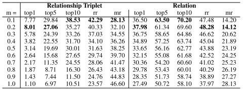
Salakhutdi-nov, and Zemel (2014); Vendrov et al. (2015); Faghri et al. (2018); Gordo and Larlus (2017)) adopted a smallmto al-low slackness during training. It is also unclear how to deter-mine the exact value ofmgiven a specific task. We follow previous works and setm= 0.2in all of our experiments.
Triplet-Softmax loss. The issue of triplet loss mentioned above can be alleviated by applying softmax on top of each triplet, i.e.:
LT rSm
x = 1 N N X i=1
−log e
s(yi,xi)
es(yi,xi)+PK
j=1e
s(yi,x−ij) (6)
LT rSmy = 1
N
N X
i=1
−log e
s(xi,yi)
es(xi,yi)+PK
j=1e
s(xi,y−ij) (7)
LT rSm=LT rSm
x +L
T rSm
y (8)
wheres(·,·)is the same similarity function (we use cosine similarity in this paper). All the other notations are the same as above. For each positive pair(xi,yi)and its
correspond-ing set of negative pairs(xi,y−ij), we calculate similarities
between each of them and put them into a softmax layer followed by multi-class logistic loss so that the similarity of positive pairs would be pushed to be1, and0otherwise. Compared to triplet loss, this loss always tries to enlarge the margin to its largest possible value (i.e., 1), thus has more discriminative power than the traditional triplet loss.
Visual Consistency loss. To further force the embeddings to be more discriminative, we add a loss that pulls closer the samples from the same category while pushes away those from different categories, i.e.:
Lc=
1 N K N X i=1 K X j=1
max[0, m+s(xi,x−ij)− min
l∈C(i)s(xi,xl)] (9)
whereN is the number of positive ROIs,C(l)is the set of positive ROIs in the same class ofxi,K is the number of
negative samplesper positiveROI andmis the margin be-tween the distances of positive and negative pairs. The in-terpretation of this loss is: the minimum similarity between samples from the same class should be larger than any sim-ilarity between samples from different classes by a margin. Here we utilize the traditional triplet loss format since we want to introduce slackness between visual embeddings to prevent embeddings from collapsing to the class centers.
Empirically we found it the best to use triplet-softmax loss for Ly while using triplet loss for Lx. The reason is simi-lar with that of the visual consistency loss: mode collapse should be prevented by introducing slackness. On the other hand, there is no such issue forysince each labelyis a mode by itself, and we encourage all modes ofyto be separated from each other. In conclusion, our final loss is:
L=LT rSm
y +αL
T r
x +βLc (10)
where we found thatα=β = 1works reasonably well for all scenarios.
Implementation details.For all the three datasets, we train our model for7epochs using 8 GPUs. We set learning rate as 0.001for the first5epochs and0.0001for the rest2epochs. We initialize each branch with weights pre-trained on COCO Lin et al. (2014). For the word vectors, we used thegensim
library ˇReh˚uˇrek and Sojka (2010) for both word2vec and node2vec1Grover and Leskovec (2016). For the triplet loss,
we setm= 0.2as the default value.
For the VRD and VG200 datasets, we need to predict whether a box pair has relationship, since unlike VG80k where we use ground-truth boxes, here we want to use gen-eral proposals that might contain non-relationships. In order for that, we add an additional “unknown” category to the re-lation categories. The word “unknown” is semantically dis-similar with any of the relations in these datasets, hence its word vector is far away from those relations’ vectors.
There is a critical factor that significantly affects our triplet-softmax loss. Since we use cosine similarity,s(·,·)is equivalent to dot product of two normalized vectors. We em-pirically found that simply feeding normalized vector could
1
cause gradient vanishing problem, since gradients are di-vided by the norm of input vector when back-propagated. This is also observed in Bell et al. (2016) where it is neces-sary to scale up normalized vectors for successful learning. Similar with Bell et al. (2016), we set the scalar to a value that is close to the mean norm of the input vectors and mul-tiplys(·,·)before feeding to the softmax layer. We set the scalar to3.2for VG80k and3.0for VRD in all experiments.
ROI Sampling.One of the critical things that powers Fast-RCNN is the well-designed ROI sampling during training. It ensures that for most ground-truth boxes, each has32 posi-tive ROIs and128−32 = 96negative ROIs, where positivity is defined as overlap IoU>= 0.5. In our setting, ROI sam-pling is similar for the subject/object branch, while for the relation branch, positivity is defined as both subject and ob-ject IoUs>= 0.5. Accordingly, we sample64subject ROIs with32unique positives and32unique negatives, and do the same thing for object ROIs. Then we pair all the64subject ROIs with 64 object ROIs to get 4096ROI pairs as rela-tionship candidates. For each candidate, if both ROIs’ IoU
>= 0.5 we mark it as positive, otherwise negative. We fi-nally sample32positive and96negative relation candidates and use the union of each ROI pair as a relation ROI. In this way we end up with a consistent number of positive and negative ROIs for the relation branch.
Experiments
Datasets. We present experiments on three datasets, the original Visual Genome (VG80k) (Krishna et al., 2017), the version ofVisual Genomewith 200 categories (VG200) (Xu et al., 2017), andVisual Relationship Detection(VRD) dataset (Lu et al., 2016).
• VRD.The VRD dataset (Lu et al., 2016) contains 5,000 images with 100 object categories and 70 relations. In to-tal, VRD contains 37,993 relation annotations with 6,672 unique relations and 24.25 relationships per object cate-gory. We follow the same train/test split as in Lu et al. (2016) to get 4,000 training images and 1,000 test im-ages. We use this dataset to demonstrate that our model can work reasonably well on small dataset with small cat-egory space, even though it is designed for large-scale set-tings.
• VG200.We also train and evaluate our model on a sub-set of VG80k which is widely used in previous methods (Xu et al., 2017; Newell and Deng, 2017; Zellers et al., 2018; Yang et al., 2018). There are totally150object cat-egories and50predicate categories in this dataset. We use the same train/test splits as in Xu et al. (2017). Similarly with VRD, the purpose here is to show our model is also state-of-the-art in large-scale sample but small-scale cate-gory settings.
• VG80k.We use the latest version of Visual Genome (VG v1.4) (Krishna et al., 2017) that contains108,077images with21 relationships on average per image. We follow Johnson, Karpathy, and Fei-Fei (2016) and split the data into103,077 training images and5,000 testing images. Since text annotations of VG are noisy, we first clean it by removing non-alphabet characters and stop words, and
use theautocorrectlibrary to correct spelling. Fol-lowing that, we check if all words in an annotation exist in the word2vec dictionary (Mikolov et al., 2013) and re-move those that do not. We run this cleaning process on both training and testing set and get99,961training im-ages and 4,871 testing images, with53,304 object cat-egories and 29,086 relation categories. We further split the training set into97,961training and2,000validation images.2
Evaluation protocol.For VRD, we use the same evaluation metrics used in Yu et al. (2017), which runs relationship de-tection using non-ground-truth proposals and reports recall rates using the top 50 and 100 relationship predictions, with
k= 1,10,70relations per relationship proposal before tak-ing the top 50 and 100 predictions.
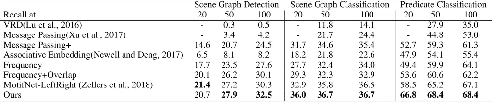
For VG200, we use the same evaluation metrics used in Zellers et al. (2018), which uses three modes: 1)predicate classification: predict predicate labels given ground truth subject and object boxes and labels; 2) scene graph clas-sification: predict subject, object and predicate labels given ground truth subject and object boxes; 3)scene graph de-tection: predict all the three labels and two boxes. Recalls under the top 20, 50, 100 predictions are used as metrics. The mean is computed over the 3 evaluation modes over R@50 and R@100 as in Zellers et al. (2018).
For VG80k, we evaluate all methods on the whole53,304 object and29,086relation categories. We use ground-truth boxes as relationship proposals, meaning there is no local-ization errors and the results directly reflect recognition abil-ity of a model. We use the following metrics to measure performance: (1) top1, top5, and top10 accuracy, (2) mean reciprocal ranking (rr), defined as M1 PM
i=1 1
ranki, (3) mean ranking (mr), defined asM1 PM
i=1ranki, smaller is better.
Evaluation of Relationship Detection on VRD
We first validate our model on VRD dataset with comparison to state-of-the-art methods using the metrics presented in Yu et al. (2017) in Table 1. Note that there is a variablekin this metric which is the number of relation candidates when se-lecting top50/100. Since not all previous methods specified
kin their evaluation, we first report performance in the “free
k” column when consideringkas a hyper-parameter that can be cross-validated. For methods where thekis reported for 1 or more values, the column reports the performance using the bestk. We then list all available results with specifickin the right two columns.
For fairness, we split the table in two parts. The top part lists methods that use the same proposals from Lu et al. (2016), while the bottom part lists methods that are based on a different set of proposals, and ours uses better pro-posals obtained from Faster-RCNN as previous works. We can see that we outperform all other methods with proposals from Lu et al. (2016) even without using message-passing-like post processing as in Li et al. (2017); Dai, Zhang, and Lin (2017), and also very competitive to the overall best per-forming method from Yu et al. (2017). Note that although
2
Relationship Phrase Relationship Detection Phrase Detection
free k k = 1 k = 10 k = 70 k = 1 k = 10 k = 70
Recall at 50 100 50 100 50 100 50 100 50 100 50 100 50 100 50 100
w/ proposals from (Lu et al., 2016)
CAI*(Zhuang et al., 2017) 15.63 17.39 17.60 19.24 - - - -Language cues(Plummer et al., 2017) 16.89 20.70 15.08 18.37 - - 16.89 20.70 - - - - 15.08 18.37 - -VRD(Lu et al., 2016) 17.43 22.03 20.42 25.52 13.80 14.70 17.43 22.03 17.35 21.51 16.17 17.03 20.42 25.52 20.04 24.90
Ours 19.18 22.64 21.69 25.92 16.08 17.07 19.18 22.64 18.89 22.35 18.32 19.78 21.69 25.92 21.39 25.65
w/ better proposals
DR-Net*(Dai, Zhang, and Lin, 2017) 17.73 20.88 19.93 23.45 - - - -ViP-CNN(Li et al., 2017) 17.32 20.01 22.78 27.91 17.32 20.01 - - - - 22.78 27.91 - - - -VRL(Liang, Lee, and Xing, 2017) 18.19 20.79 21.37 22.60 18.19 20.79 - - - - 21.37 22.60 - - - -PPRFCN*(Zhang et al., 2017b) 14.41 15.72 19.62 23.75 - - -
-VTransE* 14.07 15.20 19.42 22.42 - - -
-SA-Full*(Peyre et al., 2017) 15.80 17.10 17.90 19.50 - - - -CAI*(Zhuang et al., 2017) 20.14 23.39 23.88 25.26 - - - -KL distilation(Yu et al., 2017) 22.68 31.89 26.47 29.76 19.17 21.34 22.56 29.89 22.68 31.89 23.14 24.03 26.47 29.76 26.32 29.43 Zoom-Net(Yin et al., 2018) 21.37 27.30 29.05 37.34 18.92 21.41 - - 21.37 27.30 24.82 28.09 - - 29.05 37.34 CAI + SCA-M(Yin et al., 2018) 22.34 28.52 29.64 38.39 19.54 22.39 - - 22.34 28.52 25.21 28.89 - - 29.64 38.39
Ours 26.98 32.63 32.90 39.66 23.68 26.67 26.98 32.63 26.98 32.59 28.93 32.85 32.90 39.66 32.90 39.64
Table 1: Comparison with state-of-the-art on the VRD dataset.
Scene Graph Detection Scene Graph Classification Predicate Classification
Recall at 20 50 100 20 50 100 20 50 100
VRD(Lu et al., 2016) - 0.3 0.5 - 11.8 14.1 - 27.9 35.0
Message Passing(Xu et al., 2017) - 3.4 4.2 - 21.7 24.4 - 44.8 53.0
Message Passing+ 14.6 20.7 24.5 31.7 34.6 35.4 52.7 59.3 61.3
Associative Embedding(Newell and Deng, 2017) 6.5 8.1 8.2 18.2 21.8 22.6 47.9 54.1 55.4
Frequency 17.7 23.5 27.6 27.7 32.4 34.0 49.4 59.9 64.1
Frequency+Overlap 20.1 26.2 30.1 29.3 32.3 32.9 53.6 60.6 62.2
MotifNet-LeftRight (Zellers et al., 2018) 21.4 27.2 30.3 32.9 35.8 36.5 58.5 65.2 67.1
Ours 20.7 27.9 32.5 36.0 36.7 36.7 66.8 68.4 68.4
Table 2: Comparison with state-of-the-art on the VG200 dataset.
spatial features could be advantageous for VRD according to previous methods, we do not use them in our model in con-cern of large-scale settings. We expect better performance if integrating spatial features for VRD, but for model consis-tency we do experiments without it everywhere.
Scene Graph Classification & Detection on VG200
We present our results in Table 2. Note that scene graph clas-sification isolates the factor of subject/object localization ac-curacy by using ground truth subject/object boxes, meaning that it focuses more on the relationship recognition ability of a model, and predicate classification focuses even more on it by using ground truth subject/object boxes and labels. It is clear that the gaps between our model and others are higher on scene graph/predicate classification, meaning our model displays superior relation recognition ability.
Relationship Recognition on VG80k
Baselines.Since there is no previous method that has been evaluated in our large-scale setting, we carefully design 3 baselines to compare with. 1) 3-branch Fast-RCNN: an intu-itively straightforward model is a Fast-RCNN with a shared
conv1toconv5backbone and 3f cbranches for subject, re-lation and object respectively, where the subject and object branches share weights since they are essentially an object detector; 2) our model with softmax loss: we replace our loss with softmax loss; 3) our model with triplet loss: we replace
our loss with triplet loss.
Relationship Triplet Relation
top1 top5 top10 rr mr top1 top5 top10 rr mr
All classes
3-branch Fast-RCNN 9.73 41.95 55.19 52.10 16.36 36.00 69.59 79.83 50.77 7.81
ours w/ triplet 8.01 27.06 35.27 40.33 32.10 37.98 61.34 69.60 48.28 14.12
ours w/ softmax 14.53 46.33 57.30 55.61 16.94 49.83 76.06 82.20 61.60 8.21
ours final 15.72 48.83 59.87 57.53 15.08 52.00 79.37 85.60 64.12 6.21
Tail classes
3-branch Fast-RCNN 0.32 3.24 7.69 24.56 49.12 0.91 4.36 9.77 4.09 52.19
ours w/ triplet 0.02 0.29 0.58 7.73 83.75 0.12 0.61 1.10 0.68 86.60
ours w/ softmax 0.00 0.07 0.47 20.36 58.50 0.00 0.08 0.55 1.11 65.02
ours final 0.48 13.33 28.12 43.26 45.48 0.96 7.61 16.36 5.56 45.70
Table 3: Results on all relation classes and tail classes (#occurrence≤1024) in VG80k. Note that since VG80k is extremely imbalanced, classes with no greater than 1024 occurrences are still in the tail. In fact, there are more than 99% of relation classes but only 10.04% instances of these classes that occur for no more than 1024 times.
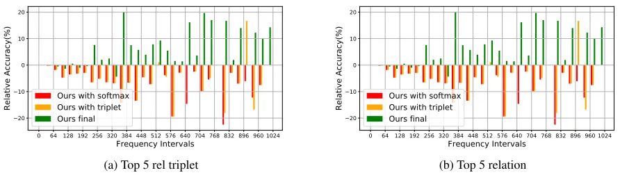
0 64 128 192 256 320 384 448 512 576 640 704 768 832 896 960 1024 Frequency Intervals
20 10 0 10 20
Relative Accuracy(%) Ours with softmaxOurs with triplet Ours final
(a) Top 5 rel triplet
0 64 128 192 256 320 384 448 512 576 640 704 768 832 896 960 1024 Frequency Intervals
20 10 0 10 20
Relative Accuracy(%) Ours with softmaxOurs with triplet Ours final
(b) Top 5 relation
Figure 3: Top-5 relative accuracies against the 3-branch Fast-RCNN baseline in the tail intervals. The intervals are defined as bins of 32 from 1 to 1024 occurrences of the relation classes.
where visual similarity is preserved. Therefore, when seeing the visual features of “dog”, “horse” and the whole “dog ride horse” context, our model is able to associate them with a vi-sually similar relationship “person ride horse” and correctly output the relation “ride”.
Ablation Study
Variants of our model.We explore variants of our model in 4 dimensions: 1) the semantic embeddings fed to the seman-tic module; 2) structure of the semanseman-tic module; 3) structure of the visual module; 4) the losses. The default settings of them are 1) usingwiki + relco; 2) 2 semantic layer; 3) with both visual concatenation; 4) with all the 3 loss terms. We fix the other 3 dimensions as the default settings when ex-ploring one of them.
The scaling factor before softmax. As mentioned in the implementation details, this value scales up the output by a value that is close to the average norm of the input and prevents gradient vanishing caused by the normaliza-tion. Specifically, for Eq(7) in the paper we uses(x,y) =
λ||xx||||Tyy|| whereλis the scaling factor. In Table 5 we show results of our model when changing the value of the scal-ing factor applied before the softmax layer. We observe that when the value is close to the average norm of all input
vec-tors (i.e., 5.0), we achieve optimal performance, although slight difference of this value does not change results too much (i.e., when it is 4.0 or 6.0). It is clear that when the scaling factor is 1.0, which is equivalent to training without scaling, the model is not sufficiently trained. We therefore pick 5.0 for this scaling factor for all the other experiments on VG80k.
Which semantic embedding to use?We explore 4 settings: 1)wikiand 2)relcouse wikipedia and relationship-level co-occurrence embedding alone, while 3)wiki + relcoand 4)
wiki + node2vecuse concatenation of two embeddings. The
intuition of concatenatingwikiwithrelco andnode2vec is that wikicontains common knowledge acquired outside of the dataset, while relco andnode2vec are trained specifi-cally on VG80k, and their combination provides abundant information for the semantic module. As shown in Table 4, fusion of wiki andrelco outperforms each one alone with clear margins. We found that usingnode2vecalone does not perform reasonably, butwiki + node2vecis competitive to others, demonstrating the efficacy of concatenation.
associa-Relationship Triplet Relation
Methods top1 top5 top10 rr mr top1 top5 top10 rr mr
wiki 15.59 46.03 54.78 52.45 25.31 51.96 78.56 84.38 63.61 8.61
relco 15.58 46.63 55.91 54.03 22.23 52.00 79.06 84.75 63.90 7.74
wiki + relco 15.72 48.83 59.87 57.53 15.08 52.00 79.37 85.60 64.12 6.21
wiki + node2vec 15.62 47.58 57.48 54.75 20.93 51.92 78.83 85.01 63.86 7.64
0 sem layer 11.21 28.78 34.84 38.64 43.49 44.66 60.06 64.74 51.60 24.74
1 sem layer 15.75 48.23 58.28 55.70 19.15 51.82 78.94 85.00 63.79 7.63
2 sem layer 15.72 48.83 59.87 57.53 15.08 52.00 79.37 85.60 64.12 6.21
3 sem layer 15.49 48.42 58.75 56.98 15.83 52.00 79.19 85.08 63.99 6.40
no concat 10.47 42.51 54.51 51.51 20.16 36.96 70.44 80.01 51.62 9.26
early concat 15.09 45.88 55.72 54.72 19.69 49.54 75.56 81.49 61.25 8.82
late concat 15.57 47.72 58.05 55.34 19.27 51.06 78.15 84.47 63.03 7.90
both concat 15.72 48.83 59.87 57.53 20.62 52.00 79.37 85.60 64.12 6.21
Ly 15.21 47.28 57.77 55.06 19.12 50.67 78.21 84.70 62.82 7.31
Ly+Lx 15.07 47.37 57.85 54.92 19.59 50.60 78.06 84.40 62.71 7.60
Ly+Lc 15.53 47.97 58.49 55.78 18.55 51.48 78.99 84.90 63.59 7.32
Ly+Lx+Lc 15.72 48.83 59.87 57.53 15.08 52.00 79.37 85.60 64.12 6.21
Table 4: Ablation study of our model on VG80k.
Relationship Triplet Relation
λ= top1 top5 top10 rr mr top1 top5 top10 rr mr 1.0 0.00 0.61 3.77 22.43 48.24 0.04 1.12 5.97 4.11 21.39 2.0 8.48 27.63 34.26 35.25 46.28 44.94 70.60 76.63 56.69 13.20 3.0 14.19 39.22 46.71 48.80 29.65 51.07 74.61 78.74 61.74 10.88 4.0 15.72 47.19 56.94 54.80 20.85 51.67 78.66 84.23 63.53 8.68 5.0 15.72 48.83 59.87 57.53 15.08 52.00 79.37 85.60 64.12 6.21
6.0 15.32 47.99 58.10 55.57 18.67 51.60 78.95 85.05 63.62 7.23 7.0 15.11 44.72 54.68 54.04 20.82 51.23 77.37 83.37 62.95 7.86 8.0 14.84 45.12 54.95 54.07 20.56 51.25 77.67 83.36 62.97 7.81 9.0 14.81 45.72 55.81 54.29 20.10 50.88 78.59 84.70 63.08 7.21 10.0 14.71 45.62 55.71 54.19 20.19 51.07 78.64 84.78 63.21 7.26
Table 5: Performances of our model on VG80k validation set with different values of the scaling factor. We use scaling factorλ= 5.0for all our experiments on VG80k.
tions between words as possible, but not to distinguish them. We find that either 1 or 2 layers give similarly good results and 2 layers are slightly better, though performance starts to degrade when adding more layers.
Are both visual feature concatenations necessary?In Ta-ble 4, “early concat” means using only the first concatena-tion of the three branches, and “late concat” means the sec-ond. Both early and late concatenation boost performance significantly compared to no concatenation, and it is the best with both. Another observation is that late concatenation is better than early alone. We believe the reason is, as men-tioned above, relations are naturally condimen-tioned on and con-strained by subjects and objects, e.g., given “man” as sub-ject and “chair” as obsub-ject, it is highly likely that the relation is “sit on”. Since late concatenation is at a higher level, it integrates features that are more semantically close to the subject and object labels, which gives stronger prior to the relation branch and affects relation prediction more than the early concatenation.
Do all the losses help?In order to understand how each loss helps training, we trained 3 models of which each excludes one or two loss terms. We can see that usingLy+Lxis
sim-ilar withLy, and it is the best with all the three losses. This
is becauseLxpulls positivexpairs close while pushes
neg-Relationship Triplet Relation
m = top1 top5 top10 rr mr top1 top5 top10 rr mr 0.1 7.77 29.84 38.53 42.29 28.13 36.50 63.50 70.20 47.48 14.20 0.2 8.01 27.06 35.27 40.33 32.10 37.98 61.34 69.60 48.28 14.12
0.3 5.78 24.39 33.26 37.03 34.55 36.75 58.65 64.86 46.62 20.62 0.4 3.82 22.55 31.70 34.10 36.26 34.89 57.25 63.74 45.04 21.89 0.5 3.14 19.69 30.01 31.63 38.25 33.65 56.16 62.77 43.88 23.19 0.6 2.64 15.68 27.65 29.74 39.70 32.15 55.08 61.68 42.52 24.25 0.7 2.17 11.35 24.55 28.06 41.47 30.36 54.20 60.60 41.02 25.23 0.8 1.87 8.71 16.30 26.43 43.18 29.78 53.43 60.01 40.29 26.19 0.9 1.43 7.44 11.50 24.76 44.83 28.35 51.73 58.74 38.89 27.27 1.0 1.10 6.97 10.51 23.57 46.60 27.49 50.72 58.10 37.97 28.13
Table 6: Performances of triplet loss on VG80k validation set with different values of margin m. We use marginm= 0.2for all our experiments in the main paper.
ativexaway. However, since(x, y)is a many-to-one map-ping (i.e., multiple visual features could have the same la-bel), there is no guarantee that allxwith the sameywould be embedded closely, if not usingLc. By introducingLc,x
with the sameyare forced to be close to each other, and thus the structural consistency of visual features is preserved.
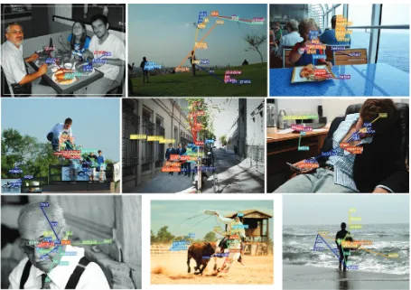
Figure 4: Qualitative results. Our model recognizes a wide range of relation ship triples. Even if they are not always matching the ground truth they are frequently correct or at least reasonable as the ground truth is not complete.
Qualitative results The VG80k has densely annotated re-lationships for most images with a wide range of types. In Figure 4 there are interactive relationships such as “boy fly-ing kite”, “batter holdfly-ing bat”, positional relationships such as “glass on table”, “man next to man”, attributive relation-ships such as “man in suit” and “boy has face”. Our model is able to cover all these kinds, no matter frequent or infre-quent, and even for those incorrect predictions, our answers are still semantic meaningful and similar to the ground-truth, e.g., the ground-truth “lamp on pole” v.s. the predicted “light on pole”, and the ground-truth “motorcycle on sidewalk” v.s. the predicted “scooter on sidewalk”.
Conclusions
In this work we study visual relationship detection at an un-precedented scale and propose a novel model that can gener-alize better on long tail class distributions. We find it is cru-cial to integrate subject and object features at multiple levels for good relation embeddings and further design a loss that learns to embed visual and semantic features into a shared space, where semantic correlations between categories are kept without hurting discriminative ability. We validate the effectiveness of our model on multiple datasets, both on the classification and detection task, and demonstrate the superi-ority of our approach over strong baselines and the
state-of-the-art. Future work includes integrating a relationship pro-posal into our model that would enable end-to-end training.
References
Bell, S.; Zitnick, C. L.; Bala, K.; and Girshick, R. 2016. Inside-outside net: Detecting objects in context with skip pooling and re-current neural networks.Computer Vision and Pattern Recognition (CVPR).
Dai, B.; Zhang, Y.; and Lin, D. 2017. Detecting visual relationships with deep relational networks. In2017 IEEE Conference on Com-puter Vision and Pattern Recognition (CVPR), 3298–3308. IEEE.
Deng, J.; Dong, W.; Socher, R.; Li, L.-J.; Li, K.; and Fei-Fei, L. 2009. Imagenet: A large-scale hierarchical image database. InComputer Vision and Pattern Recognition, 2009. CVPR 2009. IEEE Conference on, 248–255. Ieee.
Deng, J.; Ding, N.; Jia, Y.; Frome, A.; Murphy, K.; Bengio, S.; Li, Y.; Neven, H.; and Adam, H. 2014. Large-scale object clas-sification using label relation graphs. InEuropean conference on computer vision, 48–64. Springer.
Elhoseiny, M.; Cohen, S.; Chang, W.; Price, B.; and Elgammal, A. 2017. Sherlock: Scalable fact learning in images. InAAAI.
Elhoseiny, M.; Elgammal, A.; and Saleh, B. 2017. Write a classifier: Predicting visual classifiers from unstructured text.
IEEE transactions on pattern analysis and machine intelligence
Elhoseiny, M.; Saleh, B.; and Elgammal, A. 2013. Write a classi-fier: Zero-shot learning using purely textual descriptions. In Pro-ceedings of the IEEE International Conference on Computer Vi-sion, 2584–2591.
Faghri, F.; Fleet, D. J.; Kiros, J. R.; and Fidler, S. 2018. Vse++: Im-proving visual-semantic embeddings with hard negatives. In Pro-ceedings of the British Machine Vision Conference (BMVC). Frome, A.; Corrado, G. S.; Shlens, J.; Bengio, S.; Dean, J.; Mikolov, T.; et al. 2013. Devise: A deep visual-semantic embed-ding model. InAdvances in neural information processing systems, 2121–2129.
Gong, Y.; Ke, Q.; Isard, M.; and Lazebnik, S. 2014. A multi-view embedding space for modeling internet images, tags, and their semantics. International journal of computer vision106(2):210– 233.
Gordo, A., and Larlus, D. 2017. Beyond instance-level image re-trieval: Leveraging captions to learn a global visual representation for semantic retrieval. InThe IEEE Conference on Computer Vi-sion and Pattern Recognition (CVPR).
Grover, A., and Leskovec, J. 2016. node2vec: Scalable feature learning for networks. InProceedings of the 22nd ACM SIGKDD international conference on Knowledge discovery and data mining, 855–864. ACM.
Johnson, J.; Karpathy, A.; and Fei-Fei, L. 2016. Densecap: Fully convolutional localization networks for dense captioning. In Pro-ceedings of the IEEE Conference on Computer Vision and Pattern Recognition.
Kiros, R.; Salakhutdinov, R.; and Zemel, R. 2014. Multimodal neural language models. InInternational Conference on Machine Learning, 595–603.
Krishna, R.; Zhu, Y.; Groth, O.; Johnson, J.; Hata, K.; Kravitz, J.; Chen, S.; Kalantidis, Y.; Li, L.-J.; Shamma, D. A.; et al. 2017. Vi-sual genome: Connecting language and vision using crowdsourced dense image annotations. International Journal of Computer Vi-sion123(1):32–73.
Lei Ba, J.; Swersky, K.; Fidler, S.; et al. 2015. Predicting deep zero-shot convolutional neural networks using textual descriptions. InProceedings of the IEEE International Conference on Computer Vision, 4247–4255.
Li, Y.; Ouyang, W.; Wang, X.; and Tang, X. 2017. Vip-cnn: Vi-sual phrase guided convolutional neural network. InComputer Vi-sion and Pattern Recognition (CVPR), 2017 IEEE Conference on, 7244–7253. IEEE.
Liang, X.; Lee, L.; and Xing, E. P. 2017. Deep variation-structured reinforcement learning for visual relationship and attribute detec-tion.arXiv preprint arXiv:1703.03054.
Lin, T.-Y.; Maire, M.; Belongie, S.; Hays, J.; Perona, P.; Ramanan, D.; Doll´ar, P.; and Zitnick, C. L. 2014. Microsoft coco: Common objects in context. InECCV. Springer.
Lu, C.; Krishna, R.; Bernstein, M.; and Fei-Fei, L. 2016. Visual re-lationship detection with language priors. InEuropean Conference on Computer Vision, 852–869. Springer.
Mikolov, T.; Sutskever, I.; Chen, K.; Corrado, G. S.; and Dean, J. 2013. Distributed representations of words and phrases and their compositionality. InAdvances in neural information processing systems, 3111–3119.
Newell, A., and Deng, J. 2017. Pixels to graphs by associative embedding. InAdvances in neural information processing systems, 2171–2180.
Norouzi, M.; Mikolov, T.; Bengio, S.; Singer, Y.; Shlens, J.; Frome, A.; Corrado, G.; and Dean, J. 2014. Zero-shot learning by convex combination of semantic embeddings. InInternational Conference on Learning Representations.
Peyre, J.; Laptev, I.; Schmid, C.; and Sivic, J. 2017. Weakly-supervised learning of visual relations. InICCV.
Plummer, B. A.; Mallya, A.; Cervantes, C. M.; Hockenmaier, J.; and Lazebnik, S. 2017. Phrase localization and visual relationship detection with comprehensive image-language cues. In2017 IEEE International Conference on Computer Vision (ICCV), 1946–1955. IEEE.
ˇ
Reh˚uˇrek, R., and Sojka, P. 2010. Software Framework for Topic Modelling with Large Corpora. InProceedings of the LREC 2010 Workshop on New Challenges for NLP Frameworks, 45–50. Val-letta, Malta: ELRA. http://is.muni.cz/publication/884893/en. Socher, R.; Ganjoo, M.; Manning, C. D.; and Ng, A. 2013. Zero-shot learning through cross-modal transfer. InAdvances in neural information processing systems, 935–943.
Vendrov, I.; Kiros, R.; Fidler, S.; and Urtasun, R. 2015. Order-embeddings of images and language. arXiv preprint arXiv:1511.06361.
Wang, L.; Li, Y.; and Lazebnik, S. 2016. Learning deep structure-preserving image-text embeddings. InProceedings of the IEEE conference on computer vision and pattern recognition, 5005– 5013.
Xu, D.; Zhu, Y.; Choy, C. B.; and Fei-Fei, L. 2017. Scene graph generation by iterative message passing. In Proceedings of the IEEE Conference on Computer Vision and Pattern Recognition, volume 2.
Yang, J.; Lu, J.; Lee, S.; Batra, D.; and Parikh, D. 2018. Graph r-cnn for scene graph generation.arXiv preprint arXiv:1808.00191. Yin, G.; Sheng, L.; Liu, B.; Yu, N.; Wang, X.; Shao, J.; and Change Loy, C. 2018. Zoom-net: Mining deep feature interactions for visual relationship recognition. InThe European Conference on Computer Vision (ECCV).
Yu, R.; Li, A.; Morariu, V. I.; and Davis, L. S. 2017. Visual rela-tionship detection with internal and external linguistic knowledge distillation. InThe IEEE International Conference on Computer Vision (ICCV).
Zellers, R.; Yatskar, M.; Thomson, S.; and Choi, Y. 2018. Neural motifs: Scene graph parsing with global context. InConference on Computer Vision and Pattern Recognition.
Zhang, H.; Kyaw, Z.; Chang, S.-F.; and Chua, T.-S. 2017a. Vi-sual translation embedding network for viVi-sual relation detection. InComputer Vision and Pattern Recognition (CVPR), 2017 IEEE Conference on, 3107–3115. IEEE.
Zhang, H.; Kyaw, Z.; Yu, J.; and Chang, S.-F. 2017b. Ppr-fcn: Weakly supervised visual relation detection via parallel pairwise r-fcn. InProceedings of the IEEE Conference on Computer Vision and Pattern Recognition, 4233–4241.
Zhang, J.; Elhoseiny, M.; Cohen, S.; Chang, W.; and Elgammal, A. 2017c. Relationship proposal networks. In Proceedings of the IEEE Conference on Computer Vision and Pattern Recognition, 5678–5686.
Zhao, H.; Puig, X.; Zhou, B.; Fidler, S.; and Torralba, A. 2017. Open vocabulary scene parsing. InProc. IEEE Conf. Computer Vision and Pattern Recognition.
Zhuang, B.; Liu, L.; Shen, C.; and Reid, I. 2017. Towards context-aware interaction recognition for visual relationship detection. In