94
Copyright © 2011-15. Vandana Publications. All Rights Reserved.
Volume-5, Issue-3, June-2015
International Journal of Engineering and Management Research
Page Number: 94-101
Effect of Cutting Parameters in Turning of Aluminium 2024 to Obtain
Maximum MRR and Minimum Temperatue by using RSM (Under Dry
Condition)
B. Pradeep Kumar1, Dr. N.V.N. Indra Kiran.2, J.V. Bhanutej3
1, 3
Assistant Professor, Department of Mechanical Engineering, ANITS, Visakhapatnam, Andhra Pradesh, India.
2
Assoc. Professor, Department of Mechanical Engineering, ANITS, Visakhapatnam, Andhra Pradesh, India.
ABSTRACT
The main objective of this work deals with optimization of cutting parameters on aluminium 2024 specimen in turning operation to obtain Maximum Material Removal Rate(MRR), and Minimum work piece temperature using surface response analysis under dry conditions. Now a days aluminium is widely used in automobile industry, aerospace industry etc., due to its high weight to strength ratio. In the present work Full Factorial Design is considered with three process parameters: Speed, Feed and Depth of cut. By using the mathematical model the main and interaction effect of various process parameters on MRR and Temperature are studied. The developed model helps in selection of proper machining parameters for the specific material and also helps in achieving the desired Material Removal Rate and minimum Temperature.
Keywords—Material Removal Rate, Cutting Forces,
Design of Experiments, Response Surface Methodology
I.
INTRODUCTION
1.1 Turning Operation
Turning is the removal of metal from the outer diameter of a rotating cylindrical work piece. Turning is used to reduce the diameter of the work piece, usually to a specified dimension, and to produce a smooth finish on the metal. Often the work piece will be turned so that adjacent sections have different diameters. Turning is the machining operation that produces cylindrical parts.
Fig: 1.1: Parameters in turning operation
Taper turning is practically the same, except that the cutter path is at an angle to the work axis. Similarly, in contour turning, the distance of the cutter from the work axis is varied to produce the desired shape. Even though a single-point tool is specified, this does not exclude multiple-tool setup as a single-point which is often employed in turning. In such setups, each tool operates independently cutting tool.
1.2 Adjustable Cutting Parameters in Turning
The three primary factors in any basic turning operation are speed, feed, and depth of cut. Other factors such as kind of material and type of tool have a large influence, of course, but these three are the ones the operator can change by adjusting the controls, right on the machine.
1.2.1 Speed
95
Copyright © 2011-15. Vandana Publications. All Rights Reserved.
times the circumference of the work piece before the cut is started. It is expressed in meter per minute (m/min), and it refers only to the work piece. Every different diameter on a work piece will have a different cutting speed, even though the rotating speed remains the same
V= ΠDN/1000
Here, v is the cutting speed in turning in m/min,
D is the initial diameter of the work piece in mm,
N is the spindle speed in r.p.m.
1.2.2 Feed
Feed always refers to the cutting tool, and it is the rate at which the tool advances along its cutting path. On most power-fed lathes, the feed rate is directly related to the spindle speed and is expressed in mm (of tool advance) per revolution (of the spindle), or mm/rev.
Fm=f x N (mm/min) Here, Fm
1.2.3 Depth of Cut
Depth of cut is practically self explanatory. It is the thickness of the layer being removed (in a single pass) from the work piece or the distance from the uncut surface of the work to the cut surface, expressed in mm. It is important to note, though, that the diameter of the work piece is reduced by two times the depth of cut because this layer is being removed from both sides of the work
is the feed in mm per minute, f - Feed in mm/rev and
N - Spindle speed in r.p.m.
2
d
D
D
cut=
−
cut
D
- Depth of cut in mmD - Initial diameter of the work piece
d
- Final diameter of the work piece
1.3 Metal Removal Rate
It is the amount of material removed per unit time i.e., volume of material removed per unit time. Material removal rate is given by
MRR=
4 * )
(D 2 d 2 f
∏
−D is the initial diameter of the work piece d is the final diameter of the work piece f is feed in mm/min
Fig: 1.2 Metal Removal rate
1.4 High speed steels (HSS)
HSS tools are so named because they were developed to cut at higher speeds. Developed around 1900 HSS are the most highly alloyed tool steels. The tungsten (T series) was developed first and typically contains 12 - 18% tungsten, plus about 4% chromium and 17- 5% vanadium. Most grades contain about 0.5% molybdenum and most grades contain 4 - 12% cobalt.
1.5 Aluminium 2024
Studying various projects Aluminium is selected for machining operation. The composition of Aluminium 2024 is
Silicon – 0.25% Fe –0.40% Copper – 0.05% Manganese - 0.05% Magnesium – 0.05% Vanadium – 0.05% Aluminium – Remaining
The dimensions of the workpiece used are length300mm*50mmdia
II.
LITERATURE REVIEW
Dr. S. S. Chaudhari et al [1] done the investigation of a single characteristic response optimization model based on Taguchi Technique is developed to optimize process parameters, such as speed, feed, depth of cut, and nose radius of single point cutting tool. Taguchi’s L9 orthogonal array is selected for experimental planning. The experimental result analysis showed that the combination of higher levels of cutting speed, depth of cut and lower level of feed is essential to achieve simultaneous maximization of material removal rate and minimization of surface roughness. This paper also aims to determine parametric relationship and its effect on surface finish
96
Copyright © 2011-15. Vandana Publications. All Rights Reserved.
to study the effect of cutting speed, feed rate and depth of cut on Flank wear and surface roughness. Model is found to be statically significant using regression model, while feed and depth of cut are the factor affecting Flank wear and feed is dominating factors for surface roughness. The analysis of variance was used to analyse the input parameters and their interactions during machining. The developed model predicted response factor at 95% confidence level.
Ahmet Hasçalık and Ulaş Çaydaş et al[3]
studied the effect and optimization of machining parameters on surface roughness and tool life in a turning operation was investigated by using the Taguchi method. The experimental studies were conducted under varying cutting speeds, feed rates, and depths of cut. An orthogonal array, the signal-to-noise (S/N) ratio, and the analysis of variance (ANOVA) were employed to the study the performance characteristics in the turning of commercial Ti-6Al-4V alloy using CNMG 120408-883 insert cutting tools. The conclusions revealed that the feed rate and cutting speed were the most influential factors on the surface roughness and tool life, respectively. The surface roughness was chiefly related to the cutting speed, whereas the axial depth of cut had the greatest effect on tool life.
Poornima et [4] al studied Metal cutting process which is one of the complex processes which have numerous factors contributing towards the quality of the finished product. CNC turning is one among the metal cutting process in which quality of the finished product depends mainly upon the machining parameters such as feed, speed, depth of cut, type of coolant used, types of inserts used etc. Similarly the work piece material plays an important role in metal cutting process. Hard materials such as stainless steel grades, Nickel alloys, and Titanium alloys are very difficult to machine due to their high hardness. While machining these hard materials, optimized machining parameters results in good surface finish, low tool wear, etc. This study involves in identifying the optimized parameters in CNC turning of martensitic stainless steel. The optimization technique used in this study is Response surface methodology, and Genetic algorithm. These optimization techniques are very helpful in identifying the optimized control factors with high level of accuracy.
Jitendra Verma et al[5] The purpose of this research paper is focused on the analysis of optimum cutting conditions to get lowest surface roughness in turning ASTM A242 Type-1 ALLOYS STEEL by Taguchi method. Experiment was designed using Taguchi method and 9 experiments were conducted by this process. The results are analyzed using analysis of variance (ANOVA) method. Taguchi method has shown that the cutting speed has significant role to play in producing lower surface roughness about 57.47% followed by feed rate about 16.27%. The Depth of Cut has lesser role on surface roughness from the tests. The results obtained by this
method will be useful to other researches for similar type of study and may be eye opening for further research on tool vibrations, cutting forces etc.
Ishan B Shah et al[6] discuss the Optimization of tool life in milling using Design of experiment implemented to model the end milling process that are using solid carbide flat end mill as the cutting tool and stainless steels S.S-304 as material due to predict the resulting of Tool life. Data is collected from CNC milling machines were run by 8 samples of experiments using DOE approach that generate table design in MINITAB packages. The inputs of the model consist of feed, cutting speed and depth of cut while the output from the model is Tool life calculated by Taylor’s life equation. The model is validated through a comparison of the experimental values with their predicted counterparts. The optimization of the tool life is studied to compare the relationship of the parameters involve.
III.
EXPERIMENTATION
3.1 Design of Experiments
Design of Experiments is an experimental or analytical method that is commonly used to statistically signify the relationship between input parameters to output responses. DOE has wide applications especially in the field of science and engineering for the purpose of process optimization and development, process management and validation tests. DOE is essentially an experimental based modeling and is a designed experimental approach which is far superior to unplanned approach whereby a systematic way will be used to plan the experiment, collect the data and analyze the data. A mathematical model has been developed by Response Surface Methodology. Optimization and Desirability functions helps to optimize the quality characteristics considered in a DOE under a cost effective process.
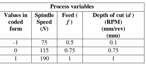
3.2 Process Variables
Three Process variables Known as factor in Design of Experiments are Speed, Feed and Depth of Cut are displayed in Table 3.1 in three levels.
Table 3.1: Process variables and their limits
Process variables Values in
coded form
Spindle Speed
(N)
Feed ( f )
Depth of cut (d ) (RPM) (mm/rev)
(mm)
-1 75 0.5 0.1
0 115 0.75 0.75
97
Copyright © 2011-15. Vandana Publications. All Rights Reserved.
3.3 Minitab Software
Minitab is a statistics package. It was developed at the Pennsylvania State University by researchers Barbara F. Ryan, Thomas A. Ryan, Jr., and Brian L. Joiner in 1972. Minitab began as a light version of MNITAB, a statistical analysis program by NIST. Minitab is distributed by Minitab Inc, a privately owned company headquartered in State College. Pennsylvania, with subsidiaries in Coventry, England, Paris, France and Sydney, Australia Today, Minitab is often used in conjunction with the implementation of Six sigma, CMMI and other statistics-based process improvement methods.
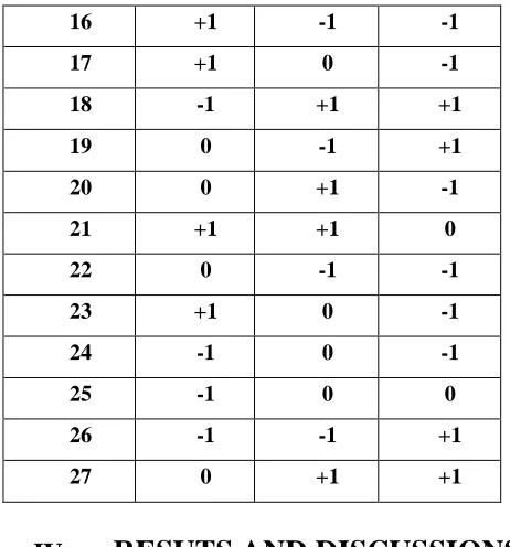
3.4 Full Factorial Method
Experiments have been carried out using full factorial method. Experimental design which consists of 27 combinations of spindle speed, longitudinal feed rate and depth of cut. According to the design catalogue prepared by factorial design of experiment has been found suitable in the present work. It considers three process parameters (without interaction) to be varied in three discrete levels. The experimental design has been shown in Table 3.2 (all factors are in coded form). Factorial design is used for conducting experiments as it allows study of interactions between factors. Interactions are the driving force in many processes.
Table 3.2 DOE in Coded form
Expt. No
Spindle
Speed
(rpm)
Feed
(mm/rev)
Depth of
cut(mm)
1 +1 0 0
2 +1 +1 -1
3 -1 0 +1
4 0 0 0
5 -1 -1 0
6 0 +1 0
7 -1 -1 -1
8 0 0 +1
9 0 -1 0
10 +1 -1 0
11 -1 +1 +1
12 +1 +1 +1
13 -1 +1 0
14 +1 -1 +1
15 0 0 -1
16 +1 -1 -1
17 +1 0 -1
18 -1 +1 +1
19 0 -1 +1
20 0 +1 -1
21 +1 +1 0
22 0 -1 -1
23 +1 0 -1
24 -1 0 -1
25 -1 0 0
26 -1 -1 +1
27 0 +1 +1
IV.
RESUTS AND DISCUSSIONS
4.1 Response Surface Methodology
Response surface methodology uses statistical models, and therefore practitioners need to be aware that even the best statistical model is an approximation to reality. In practice, both the models and the parameter values are unknown, and subject to uncertainty on top of ignorance. Of course, an estimated optimum point need not be optimum in reality, because of the errors of the estimates and of the inadequacies of the model. Nonetheless, response surface methodology has an effective track-record of helping researchers improve products and services: For example, Box's original response-surface modeling enabled chemical engineers to improve a process that had been stuck at a saddle-point for years. The engineers had not been able to afford to fit a cubic three-level design to estimate a quadratic model, and their biased linear-models estimated the gradient to be zero. Box's design reduced the costs of experimentation so that a quadratic model could be fit, which led to a (long-sought) ascent direction.
4.2 Mathematical model of Response Surface Methodology
The Response Surface is described by an second order polynomial equation of the form
Y is the corresponding response (1, 2, . . . , S) are coded levels of S quantitative process variables,
98
Copyright © 2011-15. Vandana Publications. All Rights Reserved.
Second term is attributable to linear effect, Third term corresponds to the higher-order effects, Fourth term includes the interactive effects, The last term indicates the experimental error.
4.3 Mathematical Relationship between the Input Parameters and Metal Removal Rate
The mathematical relationship for correlating the Metal removal rate and the considered process variables has been obtained as follows
MRR = 0.0321 0.000266 Speed + 0.0777 Feed 0.1659 Doc + 0.000000 Speed*Speed
- 0.1028 Feed*Feed + 0.0585 Doc*Doc + 0.000374 Speed*Feed + 0.000485 Speed*Doc + 0.1157 Feed*Doc
S. N o Speed Feed D o c M
R
R T e m p
1
7
5 0 . 5 0 . 5 0.01705653 3 0 . 6
2
7
5 0 . 5 0.75 0.021929825 3 1 . 2
3
7
5 0 . 5
1
0.029239766 3 1 . 2
4
7
5 0.75 0 . 5 0.027580772 3 1 . 5
5
7
5 0.75 0.75 0.031520883 3 0 . 8
6
7
5 0.75
1
0.047281324 3 1 . 4
7
7
5
1
0 . 5 0.024366472 3 1 . 6
8
7
5
1
0.75 0.043859649 3 1 . 6
9
7
5
1
1
0.058479532 3 4 . 6
1 0 1 1 5 0 . 5 0 . 5 0.025925926 3 0 . 0 6
1 1 1 1 5 0 . 5 0.75 0.0330033 3 1 . 8
1 2 1 1 5 0 . 5
1
0.0440044 3 1 . 8
1 3 1 1 5 0.75 0 . 5 0.040509259 3 1 . 2
1 4 1 1 5 0.75 0.75 0.052083333 3 2 . 6
1 5 1 1 5 0.75
1
0.070546737 3 2 . 2
1 6 1 1 5
1
0 . 5 0.036310821 3 1 . 2
1 7 1 1 5
1
0.75 0.058097313 3 2 . 6
1 8 1 1 5
1
1
0.087145969 3 4 . 6
1 9 1 9 0 0 . 5 0 . 5 0.047789725 3 1 . 4
2 0 1 9 0 0 . 5 0.75 0.048387097 3 1 . 8
2 1 1 9 0 0 . 5
1
0.077658303 3 1 . 8
2 2 1 9 0 0.75 0 . 5 0.058479532 3 1 . 6
2 3 1 9 0 0.75 0.75 0.087719298 3 2 . 2
2 4 1 9 0 0.75
1
0.116959064 3 2 . 6
2 5 1 9 0
1
0 . 5 0.069444444 3 2 . 1
2 6 1 9 0
1
0.75 0.09557945 3 2 . 6
2 7 1 9 0
1
1
0.131421744 3 4 . 6
4.3.1 Histogram
The Histogram is the most commonly used graph to show frequency distributions. Histograms give a rough sense of the density of the data, and often for
underlying variable. The total area of a histogram used for probability density is always normalized to 1. If the lengths of the intervals on the X-axis are all 1, then a histogram is identical to a
0.006 0.004 0.002 0.000 -0.002 -0.004 -0.006 -0.008 9 8 7 6 5 4 3 2 1 0
Residual
Fr
eq
ue
nc
y
Histogram (response is MRR)
Fig- 4.1 Histogram for MRR
4.3.2 Normal Probability Plot for MRR
The normal probability plot in the Fig:4.2 shows a clear pattern (as the points are almost in a straight line) indicating that all the factors and their interaction given in are affecting the MRR. In addition, the errors are normally distributed and the regression model is well fitted with the observed values.
0.005 0.000
-0.005 -0.010
99
95 90 80 70 60 50 40 30 20 10 5
1
Residual
Pe
rc
en
t
Normal Probability Plot (response is MRR)
Fig: 4.2 Normal Probability Plot for MRR
99
Copyright © 2011-15. Vandana Publications. All Rights Reserved.
0.140.12 0.10 0.08 0.06 0.04 0.02 0.0050
0.0025
0.0000
-0.0025
-0.0050
-0.0075
-0.0100
Fitted Value
R
es
id
ua
l
Versus Fits (response is MRR)
Fig: 4.2 Residual Vs Fitted Value for MRR
4.3.3 Effect of Input Parameters
200 150 100 0.09
0.08
0.07
0.06
0.05
0.04
0.03
1.00 0.75
0.50 0.50 0.75 1.00
Speed
M
ea
n
of
M
RR
Feed Doc
Main Effects Plot for MRR Fitted Means
Fig: 4.3 Main Effects plot for MRR
4.3.4 Interaction Effects
0.10 0.08 0.06 0.04 0.02
200 150 100 0.10 0.08 0.06 0.04 0.02
1.00 0.75
0.50 Speed * Feed
Speed * Doc
Speed
Feed * Doc
Feed
0.5 0.75 1 Feed
0.5 0.75 1 Doc
M
ea
n
of
M
RR
Interaction Plot for MRR Fitted Means
Fig: 4.4 Interaction Effects plot for MRR
4.3 Mathematical Relationship between the Input Parameters and Temperature
The mathematical relationship for correlating the Temperature and the considered process variables has been obtained as follows
Temp = 33.20 + 0.0224 Speed 9.31 Feed 5.30 Doc 0.000052 Speed*Speed + 4.41 Feed*Feed
+ 1.48 Doc*Doc 0.0030 Speed*Feed 0.0005 Speed*Doc + 8.21 Feed*Doc
4.3.1 Histogram
The Histogram is the most commonly used graph to show frequency distributions. Histograms give a rough sense of the density of the data, and often for underlying variable. The total area of a histogram used for probability density is always normalized to 1. If the lengths of the intervals on the X-axis are all 1, then a histogram is identical to a
0.75 0.50 0.25 0.00 -0.25 -0.50 -0.75 -1.00 9 8 7 6 5 4 3 2 1 0
Residual
Fr
eq
ue
nc
y
Histogram (response is Temp)
Fig- 4.5 Histogram for Temperature
4.3.2 Normal Probability Plot for Temperature
100
Copyright © 2011-15. Vandana Publications. All Rights Reserved.
1.0 0.5 0.0 -0.5 -1.0 -1.5 99 95 90 80 70 60 50 40 30 20 10 5 1 Residual Pe rc en tNormal Probability Plot (response is Temp)
Fig: 4.6 Normal Probability Plot for Temperature
4.3.2 Standardized Residual Vs Fitted Value for
Temperature
Fig: 4.7 indicates that the maximum variation which shows the high correlation that, exists between fitted values and observed values.
34.5 34.0 33.5 33.0 32.5 32.0 31.5 31.0 30.5 1.0 0.5 0.0 -0.5 -1.0 Fitted Value Re si du al Versus Fits (response is Temp)
Fig: 4.7 Residual Vs Fitted Value for Temperature
4.3.3 Effect of Input Parameters
200 150 100 33.0 32.5 32.0 31.5 31.0 1.00 0.75
0.50 0.50 0.75 1.00 Speed M ea n of T em p Feed Doc
Main Effects Plot for Temp
Fitted Means
Fig: 4.8 Main Effects plot for Temperature
4.3.4 Interaction Effects
34 33 32 31 200 150 100 34 33 32 31 1.00 0.75 0.50 Speed * Feed
Speed * Doc
Speed
Feed * Doc
Feed 0.5 0.75 1 Feed 0.5 0.75 1 Doc M ea n of T em p
Interaction Plot for Temp
Fitted Means
Fig: 4.9 Interaction Effects plot for Temperature
4.4 Optimization Plot:
A Minitab Response Optimizer tool shows how different experimental settings affect the predicted responses for factorial, response surface, and mixture designs. Minitab calculates an optimal solution and draws the plot. The optimal solution serves as the starting point for the plot. This changing the input variable settings to perform sensitivity analyses and possibly improve the initial solution.
Cur
High Low D: 0.9395Optimal Predict
d = 0.88263 Minimum
Temp
y = 32.2934
d = 1.0000 Maximum MRR
y = 0.0950
D: 0.9395 Desirability Composite 0.50 1.0 0.50 1.0 75.0
190.0 Feed Doc
Speed
[190.0] [0.6120] [1.0]
Fig: 4.10 Optimisation plot for MRR and Temperature
The optimization plot as shown in Fig: 4.10 signifies the affect of each factor (columns) on the responses or composite desirability (rows). The vertical red lines on the graph represent the current factor settings. The numbers displayed at the top of a column show the current factor level settings (in red). The horizontal blue lines and numbers represent the responses for the current factor level. Minitab calculates the maximum metal removal rate and minimum surface roughn ess.
101
Copyright © 2011-15. Vandana Publications. All Rights Reserved.
cut=0.3mm.
V. CONCLUSION
In the present work, Multi-Response Optimization problem has been solved by using an optimal parametric combination of input parameters such as Spindle speed, Feed and Depth of Cut. These optimal parameters ensures in producing high surface quality turned product.
Response Surface Methodology is successfully implemented for optimizing the input parameters.
This paper produces a direct equation with the combination of controlled parameters which can be used in industries to know the Values of MRR and Surface Roughness instead of machining.
Hence we conclude that the optimal solution for metal removal rate is 0.0950 mm3/sec and the minimum Temperature is 32.290
[3]
obtained when spindle speed=190 rpm, feed=0.612mm/rev, and depth of cut=1mm under dry conditions.
REFERENCES
[1] Dr.S.S.Chaudhari, S.S. Khedkar and N.B. Borkar. “Optimization of process parameters using Taguchi approach with minimum quantity lubrication for turning”, International Journal of Engineering Research, Vol.1 (4), 1268-1273
[2] Chetan Darshan “Analysis and Optimization of Ceramic Cutting Tool In Hard Turning of EN-31 Using Factorial Design”International Journal of Mechanical and Industrial Engineering (IJMIE), ISSN No. 2231 –6477, Vol‐1, Issue‐4, 2012
turning parameters for surface roughness and tool life based on the Taguchi method”, 2008, Volume 38
[6] Ishan B Shah, Kishore. R. Gawande ”Optimization of Cutting Tool Life on CNC Milling Machine Through Design Of Experimnets-A Suitable Approach – An overview”, International Journal of Engineering and Advanced Technology (IJEAT) ISSN: 2249 – 8958, Volume-1, Issue-4, April 2012
[7] Ajay Mishra and Dr. Anshul Gangele, 2012. “Application of Taguchi Method in Optimization of Tool
Flank Wear Width in Turning Operation of AISI 1045 Steel”, Industrial Engineering Letters, Vol. 2(8), 11-18.
pp 896-903
[4] Poornima, Sukumar “Optimization Of Machining Parameters In Cnc Turning Of Martensitic Stainless Steel Using Rsm And GA”, International Journal of Modern Engineering Research, Vol.2, Issue.2, Mar.-Apr. 2012 pp-539-542.
[5] Jitendra Verma “Turning Pameter Optimization For SurfaceRoughness Of ASTM A242 TYPE-1 Alloys Steel ByTaguchi Method”, Mechanical Engineering