419
Information Technology and Control 2018/3/47
A New State Machine
Behaviour Model for
Procedural Control Entities
in Industrial Process
Control Systems
ITC 3/47Journal of Information Technology and Control
Vol. 47 / No. 3 / 2018 pp. 419-430
DOI 10.5755/j01.itc.47.3.19630 © Kaunas University of Technology
A New State Machine Behaviour Model for Procedural Control Entities in Industrial Process Control Systems
Received 2017/12/08 Accepted after revision 2018/07/16
http://dx.doi.org/10.5755/j01.itc.47.3.19630
Corresponding author: [email protected]
Giovanni Godena, Stanko Strmčnik
Jožef Stefan Institute; Department of Systems and Control; Jamova 39, SI-1000, Ljubljana, Slovenia; phone: +386 1 477 3759; fax: +386 1 477 3994; e-mails: [email protected], [email protected]
State machines are a popular way of modelling the behaviour of systems, including process control systems. However, there are also some problems with their use in this domain, in particular in the sub-domains of the control of continuous or batch processes. The problems originate from the fact that the continuous and batch processes are, in most cases, slow in their reaction; consequently, their control sequences should have a corre-sponding duration. However, at present, all state machine models are based on instantaneous sequences, with only the loop (or do) sequence having a duration. This paper presents a new state machine behaviour model for procedural control entities in industrial process control systems. The main feature of the new concept of state machine processing is the durability of all action sequences and not only the “do” or “loop” sequence, as is the case in the existing state machine formalisms. The new concept enables modelling of control software for slow continuous or batch industrial processes in a more straightforward manner and, at the same time, on a higher level of abstraction than with using traditional state machine formalisms. The new concept is demonstrated and validated by means of a case study, which addresses a control problem from a real industrial project. The validation demonstrates that the proposed concept has a significant advantage. The concept is applicable to other classes of slow response real time systems as well.
Information Technology and Control 2018/3/47
420
1. Introduction
Industrial process control systems are hardware-soft-ware systems that control and supervise technolog-ical processes in order to achieve a process oriented goal. These systems are used in all industrial sectors because of their positive effects on productivity, prod-uct quality, flexibility, and efficiency in energy and raw material consumption. Software is the central part of process control systems because it implements vari-ous kinds of complex control activities. Interestingly, the complexity of the development, operation, and maintenance of that software is not so much associ-ated with the basic control (i.e. achieving and main-taining the desired state of the process variables), but more with so-called procedural control (i.e. perform-ing activities that ensure the achievement of the goals of the system or process). According to the estimates of Boeing and Honeywell, process control software development efforts represent 60-80% of the total control systems development engineering effort [13]; and, procedural control software represents the ma-jor and most complex part of this software. Therefore, it is of huge importance how this software is devel-oped and what its attributes are.
During the last decade a new software engineering paradigm called Model Driven Engineering (MDE) has emerged, which has the potential to sustainably raise productivity [17] and to reduce the complexity of software and systems development [20]. In MDE, the primary focus and products of software development are models rather than computer programs [21]. MDE relies on three main components, namely modelling languages, model transformations, and software tools. If models end up merely as documentation, they are of limited value. A key premise behind MDE is that programs are automatically generated from their corresponding models. Automation is by far the most effective technological means for boosting productiv-ity and reliabilproductiv-ity [21]. Hence, executable models are a key component of MDE, as well as such concepts as automatic transformation of models and validation of models [3]. Within MDE, state machines are a popu-lar way of modelling the behaviour of systems [3]. The underlying model of computation for state machines is based on the formalism of a finite state machine (FSM) [16]. FSMs are very useful for the representa-tion of reactive systems (which include process
con-trol systems), more than linear or textual notations, which are more suitable to transformational systems [15].
Although the state machine based formalisms are widely used in the modelling of process control soft-ware, there are also some problems with their use in this domain, in particular in the sub-domains of the control of continuous or batch processes. The prob-lems we have encountered during our industrial ap-plications of control systems originate from the fact that the continuous and batch processes are, in most cases, slow in their reaction; consequently, their con-trol sequences should have a corresponding duration. However, at present, all state machine models are based on instantaneous sequences, with only the loop (or do) sequence having a duration. The aim of this paper is to present a possible solution to these prob-lems and illustrate its implementation in a dedicated modelling language.
The paper is structured in the following manner. Sec-tion 2 introduces state machines and their problems in the domain of process control. Section 3 presents a possible solution to these problems in the form of a new state machine behaviour model. Section 4 gives a comparison of the traditional and the new state machine model on an industrial case study. Section 5 presents a brief discussion of the presented concept, its use, and the conclusions.
421
Information Technology and Control 2018/3/47
most common being Mealy (producing outputs along transitions) [15], Moore (producing outputs at states) [8], and a combination of these (Moore-Mealy, pro-ducing outputs both along transitions and at states). Although FSMs represent an important concept for modelling real-time behaviour, they are at a rath-er low level of abstraction in trath-erms of managing the complexity of large systems development. In the late 1980s, Harel defined a visual formalism, which he called statecharts, for describing states and transi-tions at a higher level of abstraction and in a modu-lar manner. Statecharts were essentially state tran-sition diagrams with the addition of the concepts of clustering and refinement (hierarchies of states with zoom-in and zoom-out capability), orthogonality (concurrency), and broadcast communication [8, 10]. Harel and other authors subsequently defined a pre-liminary semantics for the statechart formalism [11, 19]. Then, over the years, the statechart formalism evolved, resulting in a number of similar, though dis-tinct variants [23]. The semantics of the original con-cept was revised by Harel in 1996 and this version is often referred to in the literature as statecharts, Harel statecharts, or classical statecharts. These classical statecharts are, for instance, implemented in the tool Statemate [10, 12].
Today there are several state machine dialects, which were derived from, or at least strongly influenced by, Harel’s statecharts, e.g. UML state machines (as spec-ified in UML 2.4.1 [18]), or a newer object-oriented version of Harel’s statecharts (implemented in Rhap-sody [9]). Although the mentioned formalisms appear to be very similar, there are some subtle syntactic and semantic differences between them [3].
In the domain of process control, there are also some state machine dialects in use that are similar to those mentioned above. The most recent standard in indus-trial process control and automation systems is IEC 61499 [22], an extension of the ideas of IEC 61131-3, with support for the design phase and for distribut-ed process control systems. IEC 61499 compliant programs are based on networks of function blocks (FBs). Every FB has data inputs and outputs, which are used by the algorithms, as well as event inputs and outputs, which are used by the so-called Execu-tion Control Chart (ECC). ECC is a specific kind of statechart that defines the behaviour through the se-quencing of the algorithm invocations. Another pro-cess control approach, similar to IEC 61499 in terms
of the abstractions it uses and its expressive power, is Matlab Simulink/Stateflow. According to [2], there is a natural complementarity between the Simulink/ Stateflow and IEC 61499 Function Blocks. Simulink/ Stateflow provides a nice environment for the mod-elling and simulation of control and embedded sys-tems, while Function Blocks are good for designing distributed control systems. Additionally, Simulink/ Stateflow can also be used in the design phase, due to its C or PLC (IEC 61131-3) code generation feature. All of the above mentioned state machine formalisms are fundamentally the same concerning the basic state machine execution model. They all share a com-mon processing characteristic in which only the pro-cessing within states (i.e. loop or do propro-cessing) may have a duration, while all other processing (state entry and exit processing, and processing of transitions) is instantaneous. This model has, in our opinion, some drawbacks, particularly when considering its use in control systems of continuous or batch processes, which are in most cases slow in their reaction. With these slow systems, we would often like the entry or transition actions to take some time, e.g. to perform a device (basic control) command and then wait for it to be executed. The control software should conse-quently be executed as sequences of process actions with the duration measured in seconds, sometimes even in minutes.
A common example is the opening of an on/off valve in an entry sequence with a requirement of not to al-low the starting of the loop sequence until the action is completed. After issuing a basic control command, the sequence waits for its execution, which can take several seconds. In the current state machine formal-isms, the mentioned slow processing can be achieved by separating the processing (activities with dura-tion) from the state model, which is then just trig-gering these activities from its instantaneous actions (e.g. entry actions or transition actions). It is obvious that such a separation of behaviour and processing will likely result in difficulties caused by the neces-sary synchronisation of the completion of these ac-tivities with the starting of the loop sequence.
Information Technology and Control 2018/3/47
422
highly undesirable since Opening valve can hardly be considered as a state, especially in the frame of the process oriented view, which we would like to follow. To solve the described problem, we propose an alter-native state machine behaviour model, which is de-scribed in the next section.
3. New State Machine Behaviour
Model
In this section, a new extended state machine model for describing the dynamics of high-level control enti-ties is presented. The extension is in the introduction of a hierarchical structure of states (i.e. superstates, substates and elementary states), in fine structuring of the processing, and in the introduction of two types of transitions. The new state machine behaviour model is described by means of the state transition diagram. Syntactically, the state transition diagram is a com-bination of Venn diagrams and directed graphs. Venn diagrams are used to visualize sets and operations on them, and their only building blocks are closed curves or planar shapes. Set membership is presented with the interior of a curve. We use Venn diagrams to rep-resent sets of elements and the containment rela-tions between them. The synthesis of both notarela-tions (Venn diagrams and graphs) extends the meaning of graph vertices. The vertices appear as shapes (closed curves), which can be considered as sets in the sense of Venn diagrams (and not only as elements). In the extended state transition diagrams, the vertices can contain other vertices.
3.1. Definition of the State Transition Diagram and Its Elements
State
Syntactically, a state is a graph node denoted by a rectangle with the state name written inside. A state is shown in Figure 1.
A state transition diagram can contain different types of states, which are divided according to two criteria. According to the criterion of the processing types, the states are divided in the following way:
_ Quiescent states are states without any processing.
_ Active states are states that contain certain
processing.
According to the duration criterion, the states are di-vided in the following way:
_ Transient states are those states that contain only one sequence, and when it is executed, a transition to another state occurs. Each active transient state contains one Transient sequence.
_ Durative states are those states in which a
procedural control entity normally remains for a longer time. The processing of active durative states is divided into several sequences, which can be of different types.
A more detailed discussion on the processing of states (and transitions) is given in a separate section below. Superstate
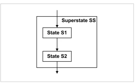
Syntactically, a superstate is a graph node denoted by a rectangle with the state name written inside. The inner area of the superstate rectangle may contain other superstates, states, and other state transition diagram elements. A superstate is shown in Figure 2.
Figure 1
State
the action is completed. After issuing a basic control command, the sequence waits for its execution, which can take several seconds. In the current state machine formalisms, the mentioned slow processing can be achieved by separating the processing (activities with duration) from the state model, which is then just triggering these activities from its instantaneous actions (e.g. entry actions or transition actions). It is obvious that such a separation of behaviour and processing will likely result in difficulties caused by the necessary synchronisation of the completion of these activities with the starting of the loop sequence.
Another possible solution in the frame of current formalisms is to introduce an additional state, called Opening valve, which has the negative consequence of lowering the granularity of state machine elements and consequently also lowering the level of abstraction. In addition, such an approach is, in our opinion, highly undesirable since Opening valve can hardly be considered as a state, especially in the frame of the process oriented view, which we would like to follow. To solve the described problem, we propose an alternative state machine behaviour model, which is described in the next section.
3. New State Machine Behaviour Model
In this section, a new extended state machine model for describing the dynamics of high-level control entities is presented. The extension is in the introduction of a hierarchical structure of states (i.e. superstates, substates and elementary states), in fine structuring of the processing, and in the introduction of two types of transitions. The new state machine behaviour model is described by means of the state transition diagram. Syntactically, the state transition diagram is a combination of Venn diagrams and directed graphs. Venn diagrams are used to visualize sets and operations on them, and their only building blocks are closed curves or planar shapes. Set membership is presented with the interior of a curve. We use Venn diagrams to represent sets of elements and the containment relations between them. The synthesis of both notations (Venn diagrams and graphs) extends the meaning of graph vertices. The vertices appear as shapes (closed curves), which can be considered as sets in the sense of Venn diagrams (and not only as elements). In the extended state transition diagrams, the vertices can contain other vertices.3.1. Definition of the State Transition Diagram and Its Elements
State
Syntactically, a state is a graph node denoted by a rectangle with the state name written inside. A state is shown in Figure 1.
State S
Figure 1 State
A state transition diagram can contain different types of states, which are divided according to two criteria. According to the criterion of the processing types, the states are divided in the following way:
• Quiescent states are states without any processing.
• Active states are states that contain certain processing.
According to the duration criterion, the states are divided in the following way:
• Transient states are those states that contain only one sequence, and when it is executed, a transition to another state occurs. Each active transient state contains one Transient sequence. • Durative states are those states in which a
procedural control entity normally remains for a longer time. The processing of active durative states is divided into several sequences, which can be of different types.
A more detailed discussion on the processing of states (and transitions) is given in a separate section below.
Superstate
Syntactically, a superstate is a graph node denoted by a rectangle with the state name written inside. The inner area of the superstate rectangle may contain other superstates, states, and other state transition diagram elements. A superstate is shown in Figure 2.
Superstate SS
State S1
State S2
Figure 2 Superstate
State diagrams are composed of a hierarchy of nested states, with superstates and substates, and with elementary states at the lowest level of the hierarchy. The purpose of nested states may be to incorporate conceptually related entities or, as the most important purpose, to avoid the repetition of information by closing into a superstate the actions and/or transitions and/or dependence relations common to a number of states. Note that a superstate is, in fact, concurrent with its active substates at all nesting levels (there may be as many concurrently active states as the number of nesting levels). In the nested states, not only pure
Figure 2
Superstate the action is completed. After issuing a basic control command, the sequence waits for its execution, which can take several seconds. In the current state machine formalisms, the mentioned slow processing can be achieved by separating the processing (activities with duration) from the state model, which is then just triggering these activities from its instantaneous actions (e.g. entry actions or transition actions). It is obvious that such a separation of behaviour and processing will likely result in difficulties caused by the necessary synchronisation of the completion of these activities with the starting of the loop sequence.
Another possible solution in the frame of current formalisms is to introduce an additional state, called Opening valve, which has the negative consequence of lowering the granularity of state machine elements and consequently also lowering the level of abstraction. In addition, such an approach is, in our opinion, highly undesirable since Opening valve can hardly be considered as a state, especially in the frame of the process oriented view, which we would like to follow. To solve the described problem, we propose an alternative state machine behaviour model, which is described in the next section.
3. New State Machine Behaviour Model
In this section, a new extended state machine model for describing the dynamics of high-level control entities is presented. The extension is in the introduction of a hierarchical structure of states (i.e. superstates, substates and elementary states), in fine structuring of the processing, and in the introduction of two types of transitions. The new state machine behaviour model is described by means of the state transition diagram. Syntactically, the state transition diagram is a combination of Venn diagrams and directed graphs. Venn diagrams are used to visualize sets and operations on them, and their only building blocks are closed curves or planar shapes. Set membership is presented with the interior of a curve. We use Venn diagrams to represent sets of elements and the containment relations between them. The synthesis of both notations (Venn diagrams and graphs) extends the meaning of graph vertices. The vertices appear as shapes (closed curves), which can be considered as sets in the sense of Venn diagrams (and not only as elements). In the extended state transition diagrams, the vertices can contain other vertices.3.1. Definition of the State Transition Diagram and Its Elements
State
Syntactically, a state is a graph node denoted by a rectangle with the state name written inside. A state is shown in Figure 1.
State S
Figure 1 State
A state transition diagram can contain different types of states, which are divided according to two criteria. According to the criterion of the processing types, the states are divided in the following way:
• Quiescent states are states without any processing.
• Active states are states that contain certain processing.
According to the duration criterion, the states are divided in the following way:
• Transient states are those states that contain only one sequence, and when it is executed, a transition to another state occurs. Each active transient state contains one Transient sequence. • Durative states are those states in which a
procedural control entity normally remains for a longer time. The processing of active durative states is divided into several sequences, which can be of different types.
A more detailed discussion on the processing of states (and transitions) is given in a separate section below.
Superstate
Syntactically, a superstate is a graph node denoted by a rectangle with the state name written inside. The inner area of the superstate rectangle may contain other superstates, states, and other state transition diagram elements. A superstate is shown in Figure 2.
Superstate SS
State S1
State S2
Figure 2 Superstate
423
Information Technology and Control 2018/3/47
important purpose, to avoid the repetition of infor-mation by closing into a superstate the actions and/ or transitions and/or dependence relations common to a number of states. Note that a superstate is, in fact, concurrent with its active substates at all nest-ing levels (there may be as many concurrently active states as the number of nesting levels). In the nested states, not only pure tree structures are possible, but also overlapping superstates. In other words, a state may be contained in one of the two superstates, or in both of them.
The proposed state machine model does not include in its current version the notion of the initial sub-state. In fact, all TO transitions are drawn explicitly to elementary states, while superstates may only have FROM transitions.
Transition “on completion”
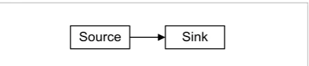
Syntactically, the transition on completion is a direct-ed line connecting an orderdirect-ed pair of nodes (source and sink), denoted by a solid line ending with an emp-ty arrowhead. Transition on completion is shown in Figure 3.
Figure 3
Transition “on completion”
tree structures are possible, but also overlapping superstates. In other words, a state may be contained in one of the two superstates, or in both of them.
The proposed state machine model does not include in its current version the notion of the initial substate. In fact, all TO transitions are drawn explicitly to elementary states, while superstates may only have FROM transitions.
Transition "on completion"
Syntactically, the transition on completion is a directed line connecting an ordered pair of nodes (source and sink), denoted by a solid line ending with an empty arrowhead. Transition on completion is shown in Figure 3.
Source Sink
Figure 3 Transition "on completion"
Transition on completion is a transition from one state (Source) to another state (Sink), which has no particular cause event, but occurs after the completion of the source state processing. According to the criterion of activity (processing), transitions on completion can be divided into active, containing activity sequences, and inactive, which have no activity sequence. A transition from a superstate cannot be "on completion". Each elementary active transient state must have exactly one FROM transition of the type "on completion".
Transition "on event"
Syntactically, the transition on event is a directed line connecting an ordered pair of nodes (source and sink), denoted by a solid line ending with a filled arrowhead. Transition on event is shown in Figure 4.
Source Sink
Figure 4 Transition "on event"
Transition on event is a transition from one state (Source) to another state (Sink), which is executed on the occurrence of a particular event. At the beginning of such a transition, first any active processing of the source state is immediately terminated. A transition from a superstate can only be of the type "on event". A transition of the type "on event" from a state S with the causing event defined by the expression State(S)=complete is equivalent to the transition "on completion" from state S.
According to the criterion of activity (processing), transitions on event, similar to those "on completion", can be divided into active, containing activity sequences, and inactive, which have no activity sequence.
3.2. Definition of the State Transition Diagram and Its Elements
The new state machine behaviour model is very finely granulated. In other words, we can say that the modelled control entities have a very finely granulated processing.
A very important feature of the processing in the new model is that all processing is composed of sequences with a duration (i.e. with non-instantaneous execution), unlike, for example, the Statecharts model, where only the Loop processing has duration, while the Entry, the Exit, and the processing of the transitions is instantaneous. The disadvantage of the latter model is in its separation of the states from the processing (actions only serve to trigger the activities, which are separated from the state model); this separation is very likely to bring difficulties with the synchronization of the activities.
As the processing of the transitions in the new state machine model has duration, and since a modelled control entity must always be in a known state, the processing of the transitions is considered as a part of the target state and is called
Specific entry processing (as it executes on the entry and is specific with respect to the source state).
The processing in the new state machine model consists of the following elements:
a. the processing of states, for each state up to one sequence of each sequence type, defined as
• ENTRY sequence, which is executed only once on entry to a given active durative state,
• LOOP sequence, which is executed
cyclically all the time while a procedural control entity is in a given active durative state (for elementary states also the opposite is true – the completion of the Loop sequence implies the completion of the state, hence the two expressions are logically equivalent: state completion ≡ Loop sequence completion),
• EXIT sequence, which is executed only once at the exit from a given active durative state,
• ALWAYS sequence, which is executed
concurrently with all activities of an active durative state, including the sequences of the transitions into that state (its specific ENTRY sequence),
• Transient sequence, which is executed only once at active transient states; and
b. sequences of the transitions into a state, which are considered as its specific Entry sequences, as stated above.
As a particular detail, let us mention at this point that the ENTRY and LOOP sequences are not executed if, at the entry to a state, the condition
Transition on completion is a transition from one state (Source) to another state (Sink), which has no particular cause event, but occurs after the comple-tion of the source state processing. According to the criterion of activity (processing), transitions on com-pletion can be divided into active, containing activity sequences, and inactive, which have no activity se-quence. A transition from a superstate cannot be “on completion”. Each elementary active transient state must have exactly one FROM transition of the type “on completion”.
Transition “on event”
Syntactically, the transition on event is a directed line connecting an ordered pair of nodes (source and sink), denoted by a solid line ending with a filled
ar-rowhead. Transition on event is shown in Figure 4.
Figure 4
Transition “on event”
tree structures are possible, but also overlapping superstates. In other words, a state may be contained in one of the two superstates, or in both of them.
The proposed state machine model does not include in its current version the notion of the initial substate. In fact, all TO transitions are drawn explicitly to elementary states, while superstates may only have FROM transitions.
Transition "on completion"
Syntactically, the transition on completion is a directed line connecting an ordered pair of nodes (source and sink), denoted by a solid line ending with an empty arrowhead. Transition on completion is shown in Figure 3.
Source Sink
Figure 3 Transition "on completion"
Transition on completion is a transition from one state (Source) to another state (Sink), which has no particular cause event, but occurs after the completion of the source state processing. According to the criterion of activity (processing), transitions on completion can be divided into active, containing activity sequences, and inactive, which have no activity sequence. A transition from a superstate cannot be "on completion". Each elementary active transient state must have exactly one FROM transition of the type "on completion".
Transition "on event"
Syntactically, the transition on event is a directed line connecting an ordered pair of nodes (source and sink), denoted by a solid line ending with a filled arrowhead. Transition on event is shown in Figure 4.
Source Sink
Figure 4 Transition "on event"
Transition on event is a transition from one state (Source) to another state (Sink), which is executed on the occurrence of a particular event. At the beginning of such a transition, first any active processing of the source state is immediately terminated. A transition from a superstate can only be of the type "on event". A transition of the type "on event" from a state S with the causing event defined by the expression State(S)=complete is equivalent to the transition "on completion" from state S.
According to the criterion of activity (processing), transitions on event, similar to those "on completion", can be divided into active, containing activity sequences, and inactive, which have no activity sequence.
3.2. Definition of the State Transition Diagram and Its Elements
The new state machine behaviour model is very finely granulated. In other words, we can say that the modelled control entities have a very finely granulated processing.
A very important feature of the processing in the new model is that all processing is composed of sequences with a duration (i.e. with non-instantaneous execution), unlike, for example, the Statecharts model, where only the Loop processing has duration, while the Entry, the Exit, and the processing of the transitions is instantaneous. The disadvantage of the latter model is in its separation of the states from the processing (actions only serve to trigger the activities, which are separated from the state model); this separation is very likely to bring difficulties with the synchronization of the activities.
As the processing of the transitions in the new state machine model has duration, and since a modelled control entity must always be in a known state, the processing of the transitions is considered as a part of the target state and is called
Specific entry processing (as it executes on the entry and is specific with respect to the source state).
The processing in the new state machine model consists of the following elements:
a. the processing of states, for each state up to one sequence of each sequence type, defined as
• ENTRY sequence, which is executed only once on entry to a given active durative state,
• LOOP sequence, which is executed
cyclically all the time while a procedural control entity is in a given active durative state (for elementary states also the opposite is true – the completion of the Loop sequence implies the completion of the state, hence the two expressions are logically equivalent: state completion ≡ Loop sequence completion),
• EXIT sequence, which is executed only once at the exit from a given active durative state,
• ALWAYS sequence, which is executed
concurrently with all activities of an active durative state, including the sequences of the transitions into that state (its specific ENTRY sequence),
• Transient sequence, which is executed only once at active transient states; and
b. sequences of the transitions into a state, which are considered as its specific Entry sequences, as stated above.
As a particular detail, let us mention at this point that the ENTRY and LOOP sequences are not executed if, at the entry to a state, the condition
Transition on event is a transition from one state (Source) to another state (Sink), which is executed on the occurrence of a particular event. At the begin-ning of such a transition, first any active processing of the source state is immediately terminated. A tran-sition from a superstate can only be of the type “on event”. A transition of the type “on event” from a state S with the causing event defined by the expression State(S)=complete is equivalent to the transition “on completion” from state S.
According to the criterion of activity (processing), transitions on event, similar to those “on comple-tion”, can be divided into active, containing activity sequences, and inactive, which have no activity se-quence.
3.2. Definition of the State Transition Diagram and Its Elements
The new state machine behaviour model is very finely granulated. In other words, we can say that the mod-elled control entities have a very finely granulated processing.
A very important feature of the processing in the new model is that all processing is composed of sequenc-es with a duration (i.e. with non-instantaneous exe-cution), unlike, for example, the Statecharts model, where only the Loop processing has duration, while the Entry, the Exit, and the processing of the transi-tions is instantaneous. The disadvantage of the latter model is in its separation of the states from the pro-cessing (actions only serve to trigger the activities, which are separated from the state model); this sep-aration is very likely to bring difficulties with the syn-chronization of the activities.
Information Technology and Control 2018/3/47
424
processing of the transitions is considered as a part of the target state and is called Specific entry process-ing (as it executes on the entry and is specific with re-spect to the source state).
The processing in the new state machine model con-sists of the following elements:
a the processing of states, for each state up to one
se-quence of each sese-quence type, defined as
_ ENTRY sequence, which is executed only once
on entry to a given active durative state,
_ LOOP sequence, which is executed cyclically all
the time while a procedural control entity is in a given active durative state (for elementary states also the opposite is true – the completion of the Loop sequence implies the completion of the state, hence the two expressions are logically equivalent: state completion ≡ Loop sequence completion),
_ EXIT sequence, which is executed only once at the exit from a given active durative state,
_ ALWAYS sequence, which is executed
concur-rently with all activities of an active durative state, including the sequences of the transitions into that state (its specific ENTRY sequences),
_ Transient sequence, which is executed only once at active transient states; and
b sequences of the transitions into a state, which are considered as its specific Entry sequences, as stat-ed above.
As a particular detail, let us mention at this point that the ENTRY and LOOP sequences are not executed if, at the entry to a state, the condition for its termina-tion is satisfied; however, the EXIT sequence is exe-cuted in every case.
3.3. State Machine Execution
Transitions firing susceptibility
The firing susceptibility of transition T1 begins when the processing of transition T2 traverses the source state of transition T1. In terms of processing sequenc-es, the transition becomes susceptible after enabling the Always processing and before starting the transi-tion’s source state Entry sequence (if source state is a superstate, Figure 5a), or before starting the tran-sition’s source state Specific entry sequence, that is the sequence of the transition T2 (if source state is an elementary state, Figure 5b).
The firing susceptibility of transition T1 ends when the processing of transition T2 traverses the source state of transition T1, or just before starting transi-tion’s source state Exit sequence (Figure 6a). The ing susceptibility of transition T1 also ends on the fir-ing of transition T2 from the same state (Figure 6b).
Figure 5
Begin of firing susceptibility
Figure 6
End of firing susceptibility
for its termination is satisfied; however, the EXIT sequence is executed in every case.
3.3. State Machine Execution Transitions firing susceptibility
The firing susceptibility of transition T1 begins when the processing of transition T2 traverses the source state of transition T1. In terms of processing sequences, the transition becomes susceptible after enabling the Always processing and before starting the transition's source state Entry sequence (if source state is a superstate, Figure 5a), or before starting the transition's source state Specific entry sequence, that is the sequence of the transition T2 (if source state is an elementary state, Figure 5b).
T2 T1
a)
T2 T1
b)
Figure 5 Begin of firing susceptibility
The firing susceptibility of transition T1 ends when the processing of transition T2 traverses the source state of transition T1, or just before starting transition's source state Exit sequence (Figure 6a). The firing susceptibility of transition T1 also ends on the firing of transition T2 from the same state (Figure 6b).
T2 T1
a)
T2 T1
b)
Figure 6 End of firing susceptibility
Transitions priorities
If the transition conditions for more susceptible transitions become true at a given moment, the transition with the highest priority position will be activated according to the following rules:
1. Transitions caused by propagations have higher priority than ordinary transitions.
2. Among transitions at different levels in the hierarchy of states, higher priority is assigned to transitions with the source in higher-level (outer) superstates. 3. Among transitions with the sources at the same level
in the hierarchy of states, higher priority is assigned to transitions with the sink in higher-level (outer)
superstates.
4. If the transition conditions for more susceptible transitions with both sources and sinks at the same level become true at a given moment, the choice of a transition to be fired is non-deterministic.
The sequence of processing on state transition Before giving the definition of the sequence of processing on state transition, we shall define the term of the root state. The root state is the elementary state, active at the time of transition firing, that is the source state or a substate of the source state, in case that the source state is a superstate. The sequence of processing on state transition from a source state to a target state is as follows:
1. The processing of all substates of the source state is terminated. This includes all Entry, Loop, Exit, and Always processing and the processing of transitions into the target state (specific Entry processing) of all substates. 2. On the path from the source to the sink state,
first for the source state, and then successively, following the increasing state hierarchy for each superstate of the root state that is not a superstate of the target state, the following successive steps are performed:
a) termination of the Entry, Loop, Transient and Specific entry processing,
b) execution (starting and waiting for completion) of the Exit processing,
c) termination of the Always processing. 3. The state variable value changes from the
source to the sink state.
4. On the path from the source to the sink state, following the decreasing state hierarchy for each superstate of the sink state that is not a superstate of the root state, the following successive steps are performed:
a) enabling the Always processing,
b) execution (starting and waiting for completion) of the Entry processing,
c) enabling the Loop processing.
5. For the sink state, the following successive steps are performed:
a) enabling the Always processing,
b) execution (starting and waiting for completion) of the Specific entry processing (the processing of the transition into the sink state),
c) execution (starting and waiting for completion) of the Entry processing,
d) enabling the Loop processing.
If the sink state is a transient state, then instead of c) and d), there is an execution (starting and
a
a b
b
for its termination is satisfied; however, the EXIT sequence is executed in every case.
3.3. State Machine Execution
Transitions firing susceptibilityThe firing susceptibility of transition T1 begins when the processing of transition T2 traverses the source state of transition T1. In terms of processing sequences, the transition becomes susceptible after enabling the Always processing and before starting the transition's source state Entry sequence (if source state is a superstate, Figure 5a), or before starting the transition's source state Specific entry sequence, that is the sequence of the transition T2 (if source state is an elementary state, Figure 5b).
T2 T1
a)
T2 T1
b)
Figure 5 Begin of firing susceptibility
The firing susceptibility of transition T1 ends when the processing of transition T2 traverses the source state of transition T1, or just before starting transition's source state Exit sequence (Figure 6a). The firing susceptibility of transition T1 also ends on the firing of transition T2 from the same state (Figure 6b).
T2 T1
a)
T2 T1
b)
Figure 6 End of firing susceptibility
Transitions priorities
If the transition conditions for more susceptible transitions become true at a given moment, the transition with the highest priority position will be activated according to the following rules:
1. Transitions caused by propagations have higher priority than ordinary transitions.
2. Among transitions at different levels in the hierarchy of states, higher priority is assigned to transitions with the source in higher-level (outer) superstates. 3. Among transitions with the sources at the same level
in the hierarchy of states, higher priority is assigned to transitions with the sink in higher-level (outer)
superstates.
4. If the transition conditions for more susceptible transitions with both sources and sinks at the same level become true at a given moment, the choice of a transition to be fired is non-deterministic.
The sequence of processing on state transition Before giving the definition of the sequence of processing on state transition, we shall define the term of the root state. The root state is the elementary state, active at the time of transition firing, that is the source state or a substate of the source state, in case that the source state is a superstate. The sequence of processing on state transition from a source state to a target state is as follows:
1. The processing of all substates of the source state is terminated. This includes all Entry, Loop, Exit, and Always processing and the processing of transitions into the target state (specific Entry processing) of all substates. 2. On the path from the source to the sink state,
first for the source state, and then successively, following the increasing state hierarchy for each superstate of the root state that is not a superstate of the target state, the following successive steps are performed:
a) termination of the Entry, Loop, Transient and Specific entry processing,
b) execution (starting and waiting for completion) of the Exit processing,
c) termination of the Always processing.
3. The state variable value changes from the source to the sink state.
4. On the path from the source to the sink state, following the decreasing state hierarchy for each superstate of the sink state that is not a superstate of the root state, the following successive steps are performed:
a) enabling the Always processing,
b) execution (starting and waiting for completion) of the Entry processing,
c) enabling the Loop processing.
5. For the sink state, the following successive steps are performed:
a) enabling the Always processing,
b) execution (starting and waiting for completion) of the Specific entry processing (the processing of the transition into the sink state),
c) execution (starting and waiting for completion) of the Entry processing,
d) enabling the Loop processing.
If the sink state is a transient state, then instead of c) and d), there is an execution (starting and
Transitions priorities
If the transition conditions for more susceptible tran-sitions become true at a given moment, the transition with the highest priority position will be activated ac-cording to the following rules:
1 Transitions caused by propagations have higher
priority than ordinary transitions.
2 Among transitions at different levels in the
hierar-chy of states, higher priority is assigned to transi-tions with the source in higher-level (outer) super-states.
425
Information Technology and Control 2018/3/47
level in the hierarchy of states, higher priority is as-signed to transitions with the sink in higher-level (outer) superstates.
4 If the transition conditions for more susceptible
transitions with both sources and sinks at the same level become true at a given moment, the choice of a transition to be fired is non-deterministic. The sequence of processing on state transition Before giving the definition of the sequence of pro-cessing on state transition, we shall define the term of the root state. The root state is the elementary state, active at the time of transition firing, that is the source state or a substate of the source state, in case that the source state is a superstate. The sequence of processing on state transition from a source state to a target state is as follows:
1 The processing of all substates of the source state is terminated. This includes all Entry, Loop, Exit, and Always processing and the processing of tran-sitions into the target state (specific Entry process-ing) of all substates.
2 On the path from the source to the sink state, first
for the source state, and then successively, follow-ing the increasfollow-ing state hierarchy for each super-state of the root super-state that is not a supersuper-state of the target state, the following successive steps are per-formed:
a termination of the Entry, Loop, Transient and
Specific entry processing,
b execution (starting and waiting for completion)
of the Exit processing,
c termination of the Always processing.
3 The state variable value changes from the source to
the sink state.
4 On the path from the source to the sink state,
fol-lowing the decreasing state hierarchy for each su-perstate of the sink state that is not a susu-perstate of the root state, the following successive steps are performed:
a enabling the Always processing,
b execution (starting and waiting for completion)
of the Entry processing,
c enabling the Loop processing.
5 For the sink state, the following successive steps
are performed:
a enabling the Always processing,
b execution (starting and waiting for completion)
of the Specific entry processing (the processing of the transition into the sink state),
c execution (starting and waiting for completion)
of the Entry processing,
d enabling the Loop processing.
If the sink state is a transient state, then instead of c) and d), there is an execution (starting and waiting for completion) of its Transient processing.
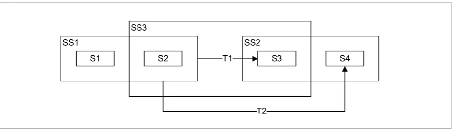
The new state machine behaviour model allows over-lapping of superstates. For an illustration of the impli-cations of this fact, let us consider a few examples of state transitions in state machines including super-states, which are shown in Figure 7. In the example, the firing of a transition has the following implications on the activation or deactivation of individual superstates.
1 Transition T1 implies activity of elementary state
S3 and superstates SS2 and SS3. At the transition,
Figure 7
An illustration of state transitions including overlapping superstates
waiting for completion) of its Transient processing. The new state machine behaviour model allows overlapping of superstates. For an illustration of the implications of this fact, let us consider a few examples of state transitions in state machines including superstates, which are shown in Figure 7. In the example, the firing of a transition has the following implications on the activation or deactivation of individual superstates.
1. Transition T1 implies activity of elementary state S3 and superstates SS2 and SS3. At the transition, the superstate SS2 has to be activated, while the possible need of the activation of SS3 depends on which elementary state was active at the time of transition firing, as follows:
• if elementary state S1 was active ⇒ superstate SS3 is activated, since it has to be active concurrently with state S3, which is the next active elementary state;
• if elementary state S2 was active ⇒ superstate SS3 is not activated, since it already was active, being a superstate of S2.
2. Transition T2 implies activity of elementary state S4 and superstate SS2. At the transition, the possible need of the deactivation of SS3 is dependent on which elementary state was active at the time of transition firing, as follows:
• if elementary state S1 was active ⇒ superstate SS3 is not deactivated, since it already was non-active, not being a superstate of S1;
• if elementary state S2 was active ⇒ superstate SS3 is deactivated, since it was active concurrently with S2, being its superstate, and it should not be active concurrently with S4, not being its superstate.
4. A Comparison of the Traditional and
the New State Machine Model on an
Industrial Case Study
The proposed new state machine behaviour model has been implemented in the domain specific modelling
language ProcGraph. The language is a part of a MDE based development methodology described in [6]. An earlier version of ProcGraph was described in [4]. Various versions of ProcGraph have been successfully used over the last fifteen years in more than twenty industrial projects, ranging in size (expressed in a commonly used number-of-signals-based metrics) from a couple of hundred to a couple of thousand signals. Some of the most interesting projects include PVA glue production, resin synthesis in paint and varnish production, and several sub-processes of the titanium dioxide production process (ore grinding, ore digestion, hydrolysis, calcinate grinding, gel washing, chemical treatment, pigment washing, pigment drying, and pigment micronisation). Let us also note that a very similar version of a state machine behaviour model, adapted to batch process control software, has been implemented in a tool for batch process control on a PLC platform, called PLCbatch [5, 7].
In the following, we give an illustration of the new behaviour model using one of the sub-processes of the above-mentioned titanium dioxide production process.
4.1. A Short Introduction of the Industrial Process Considered in the Example
Titanium dioxide (TiO2) is a white pigment that is widely used in paint and enamel production. The production of the TiO2 pigment in the Cinkarna chemical works consists of a succession of several processes. One of the sub-processes in the first stage of the production (the so-called black part of the production) is the batch process of ore digestion. In fact, it is the second sub-process, the first being the ore grinding sub-process. The ore digestion sub-process has both batch and continuous processing. The continuous part is dealing with the transport of various input materials (ore, concentrated sulfuric acid, weak acid, washing water, etc.). The batch part consists of six digester units and a common vessel for pre-mixing ore and concentrated sulfuric acid. SS3
SS2 SS1
S1 S2 T1 S3 S4
T2
Information Technology and Control 2018/3/47
426
the superstate SS2 has to be activated, while the possible need of the activation of SS3 depends on which elementary state was active at the time of transition firing, as follows:
_ if elementary state S1 was active ⇒ superstate SS3
is activated, since it has to be active concurrently with state S3, which is the next active elementary state;
_ if elementary state S2 was active ⇒ superstate SS3 is not activated, since it already was active, being a superstate of S2.
2 Transition T2 implies activity of elementary state S4 and superstate SS2. At the transition, the pos-sible need of the deactivation of SS3 is dependent on which elementary state was active at the time of transition firing, as follows:
_ if elementary state S1 was active ⇒ superstate SS3 is not deactivated, since it already was non-active, not being a superstate of S1;
_ if elementary state S2 was active ⇒ superstate SS3
is deactivated, since it was active concurrently with S2, being its superstate, and it should not be active concurrently with S4, not being its superstate.
4.
A Comparison of the Traditional
and the New State Machine Model
on an Industrial Case Study
The proposed new state machine behaviour model has been implemented in the domain specific model-ling language ProcGraph. The language is a part of a MDE based development methodology described in [6]. An earlier version of ProcGraph was described in [4]. Various versions of ProcGraph have been suc-cessfully used over the last fifteen years in more than twenty industrial projects, ranging in size (expressed in a commonly used number-of-signals-based met-rics) from a couple of hundred to a couple of thousand signals. Some of the most interesting projects include PVA glue production, resin synthesis in paint and var-nish production, and several sub-processes of the ti-tanium dioxide production process (ore grinding, ore digestion, hydrolysis, calcinate grinding, gel washing, chemical treatment, pigment washing, pigment dry-ing, and pigment micronisation). Let us also note that a very similar version of a state machine behaviour
model, adapted to batch process control software, has been implemented in a tool for batch process control on a PLC platform, called PLCbatch [5, 7].
In the following, we give an illustration of the new be-haviour model using one of the sub-processes of the above-mentioned titanium dioxide production process.
4.1. A Short Introduction of the Industrial Process Considered in the Example
Titanium dioxide (TiO2) is a white pigment that is
widely used in paint and enamel production. The pro-duction of the TiO2 pigment in the Cinkarna chemical
works consists of a succession of several processes. One of the sub-processes in the first stage of the pro-duction (the so-called black part of the propro-duction) is the batch process of ore digestion. In fact, it is the second sub-process, the first being the ore grinding sub-process. The ore digestion sub-process has both batch and continuous processing. The continuous part is dealing with the transport of various input materials (ore, concentrated sulfuric acid, weak acid, washing water, etc.). The batch part consists of six di-gester units and a common vessel for pre-mixing ore and concentrated sulfuric acid.
For the purpose of illustration, a continuous opera-tion of pneumatic transport of the ground ore from the ground ore storage silo into the pre-mixing ves-sel dosing silo was used. The pneumatic transport is performed by means of a fluidisation vessel, which is situated beneath the storage silo. During the trans-port, the fluidisation vessel is alternately filled and emptied by means of compressed air, which pushes the ore through the pipeline towards the dosing silo. Once inside the dosing silo, most of the ore falls to the bottom, while some remains on the bag filters at the top of the silo, while the air passes through the filters and it is released into the atmosphere.
In the illustration, we point out the difference be-tween two versions of a selected behaviour, namely the version that has been produced by using the new be-haviour model and the version that would be produced if the usual state machine behaviour model was used.
4.2. Use of the New State Machine Model
427
Information Technology and Control 2018/3/47
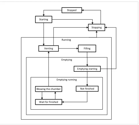
Stopping. The state Running is a superstate, which is composed of three states, namely elementary states Venting and Filling, and a superstate Emptying (of the fluidisation vessel). The Emptying superstate is composed of two states, namely an elementary state Emptying starting and a superstate Emptying run-ning, which is composed of three elementary states, namely Not finished, Wait for finished, and Blowing the chamber. As we can see, the behaviour of the op-eration is quite simple, and the states are rather intu-itive and self-explanatory.
Figure 8
Pneumatic transport state machine according to the new model For the purpose of illustration, a continuous operation of pneumatic transport of the ground ore from the ground ore storage silo into the pre-mixing vessel dosing silo was used. The pneumatic transport is performed by means of a fluidisation vessel, which is situated beneath the storage silo. During the transport, the fluidisation vessel is alternately filled and emptied by means of compressed air, which pushes the ore through the pipeline towards the dosing silo. Once inside the dosing silo, most of the ore falls to the bottom, while some remains on the bag filters at the top of the silo, while the air passes through the filters and it is released into the atmosphere.
In the illustration, we point out the difference between two versions of a selected behaviour, namely the version that has been produced by using the new behaviour model and the version that would be produced if the usual state machine behaviour model was used.
4.2. Use of the New State Machine Model
The state machine of the pneumatic transport operation according to the new model is shown in Figure 8.
The state machine has typical states of a continuous operation, namely Stopped, Starting, Running, and Stopping. The state Running is a superstate, which is composed of three states, namely elementary states Venting and Filling, and a superstate Emptying (of the fluidisation vessel). The Emptying superstate is composed of two states, namely an elementary state Emptying starting and a superstate Emptying running, which is composed of three elementary states, namely Not finished, Wait for finished, and Blowing the chamber. As we can see, the behaviour of the operation is quite simple, and the states are rather
Running
Emptying
Emptying running Stopped
Venting
Emptying starting
Not finished
Wait for finished Starting
Stopping
Blowing the chamber
Filling
Figure 8 Pneumatic transport state machine according to the new model
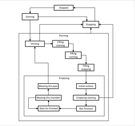
4.3. Use of the Traditional State Machine Model
Let us see now the state machine of the pneumatic transport operation as it would be if the traditional state machine model was used. This state machine is shown in Figure 9.
Information Technology and Control 2018/3/47
428
Figure 9
Pneumatic transport state machine according to the traditional model intuitive and self-explanatory.
4.3. Use of the Traditional State Machine Model
Let us see now the state machine of the pneumatic transport operation as it would be if the traditional state machine model was used. This state machine is shown in Figure 9.
It is obvious that the state diagram in this case is more complex due to a larger number of elementary states. In fact, the Running superstate in this case has 10 elementary sub-states, while in the case when the new behaviour model was used, the number of these sub-states was just 6, as can be seen in Figure 8.
4.4. Comparison of Both State Machine
Models
In the following, we point out the differences between the two state machines and give an explanation of these differences. There are three points where these differences arise.
The first difference is the state Filling (see Figure 8). This state's processing is composed of three parts, each of them having duration. The first part includes the filling starting sequence, which has a duration due to a number of sub-sequences it is composed of, where each sub-sequence has to be completed before proceeding to the next sub-sequence. The second part includes waiting for the filling of the chamber to be completed, which also takes some time. Finally, the third part, including the filling stopping sequence, also has a duration,
Running
Emptying Stopped
Filling stopping Venting
Initial actions
Emptying starting
Not finished Wait for finished
Blowing the pipe Starting
Stopping
Blowing the chamber Filling starting
Filling running
Figure 9 Pneumatic transport state machine according to the traditional model
behaviour model was used, the number of these sub-states was just 6, as can be seen in Figure 8.
4.4. Comparison of Both State Machine Models
In the following, we point out the differences between the two state machines and give an explanation of these differences. There are three points where these differences arise.
The first difference is the state Filling (see Figure 8).
start-429
Information Technology and Control 2018/3/47
ing sequence. The new state machine behaviour mod-el has enabled us to pack all three durative sequences into just one state by allocating the filling starting se-quence to the state’s Entry sese-quence, the waiting for the completion of filling to the Loop sequence, and the filling stopping sequence to the state’s Exit sequence. Since in the traditional state behaviour model only Loop processing may have duration, the Filling pro-cessing had to be allocated to three distinct states, as shown in Figure 9, namely Filling starting, Filling running, and Filling stopping.
The second difference is in the elementary state Initial actions (a sub-state of the Emptying state), which ap-pears in the state machine according to the traditional model in Figure 9, while in the state machine accord-ing to the new model in Figure 8, this state seems to be missing. But this is not the case, as its functionality has now been allocated to the Entry sequence of the Emptying state, where it fits best due to the fact that these initial actions are, in fact, initial actions of the Emptying state. In the traditional model, placing this functionality to that point is not possible, since this se-quence has duration and states’ Entry sese-quences in the traditional model cannot have duration.
The third difference is in the elementary state Blow-ing the pipe (a sub-state of the EmptyBlow-ing state), which appears in the state machine according to the tradi-tional model in Figure 9, while in the state machine according to the new model in Figure 8, this state also seems to be missing. Actually, however, its functional-ity has now been allocated to the Exit sequence of the Emptying running state. In the traditional model, plac-ing this functionality to that point is not possible, since this sequence has a duration and states’ Exit sequences in the traditional model cannot have duration. For that reason, this functionality was placed into a distinct state Blowing the pipe, while the superstate Emptying running was omitted, since there was no other pro-cessing to be allocated to this state. Omitting this state could be considered as another drawback of the state machine in Figure 9, since the Emptying superstate is
now composed of just six flat elementary states, which represents a certain lack of structure.
The above comparison clearly illustrates the advan-tages of the proposed new model, which was success-fully used in a number of industrial applications.
5. Conclusion
In this paper, a new extended state machine behaviour model for industrial process control systems was de-scribed. The extension is in the introduction of a hi-erarchical structure of states, in a fine structuring of the processing, and in the introduction of two types of transitions. The main feature of the new concept of processing is the durability of all actions sequences – not only the do or loop sequence – as is the case of other state machine formalisms. This enables modelling of control software for slow continuous or batch indus-trial processes in a more straightforward manner and, at the same time, on a higher level of abstraction than with using traditional state machine abstractions. Our experiences with the use of the proposed be-haviour model in real industrial projects are very pos-itive, and, in our opinion, the new model has a great potential to improve the quality and the complexity management of process control software.
The new concept has been implemented in a do-main-specific modelling language, ProcGraph, which has been successfully used in a number of small- and medium-sized industrial automation projects. The concept has been developed for and demonstrat-ed in the domain of industrial process control sys-tems; however, it could be applied with benefit to any class of slow response real time (reactive) systems.
Acknowledgement
The financial support of the Slovenian Research Agency (ARRS) is gratefully acknowledged.
References
1. Booch, G., Jacobson, I. Rumbaugh, J. The Unified Mod-elling Language User Guide, Addison Wesley, 1999. 2. Chia-han, Y., Vyatkin, V. Model Transformation
Be-tween MATLAB Simulink and Function Blocks.
Pro-ceedings of IEEE International Conference on Indus-trial Informatics (INDIN’10), Osaka, Japan, IEEE, 2010, 1130-1135.
Rhap-Information Technology and Control 2018/3/47
430
sody Statecharts: Not All Models Are Created Equal. Software and Systems Modeling, 2007, 6(4), 415-435. https://doi.org/10.1007/s10270-006-0042-8
4. Godena, G. ProcGraph: A Procedure-Oriented Graph-ical Notation for Process-Control Software Specifica-tion. Control Engineering Practice, 2004, 12(1), 99-111. https://doi.org/10.1016/S0967-0661(03)00002-9 5. Godena, G. A New Proposal for the Behaviour Model of
Batch Phases. ISA Transactions, 2009, 48, 3-9. https:// doi.org/10.1016/j.isatra.2008.08.002
6. Godena, G., Lukman, T., Kandare, G. A New Approach to Control Systems Software Development. In: Strmčnik, S., Juričić, Đ. (Eds.), Case Studies in Control: Putting Theory to Work, (Advances in Industrial Control, ISSN 1430-9491). London [etc.]: Springer, 2013, 363-406. 7. Godena, G., Steiner, I., Tancek, J., Svetina, M. Design of a
Batch Process Control Tool on the Programmable Log-ic Controller Platform. In: Hawkins, William M. (Ed.), Brandl, Dennis (Ed.), Boyes, Walt (Eds.). ISA-88 Imple-mentation Experiences, (The WBF Book Series, vol. 1). New York: Momentum Press, 2010, 157-173.
8. Harel, D. Statecharts: A Visual Formalism for Complex Systems. Science of Computer Programming, 1987, 8(3), 231-274. https://doi.org/10.1016/0167-6423(87)90035-9 9. Harel, D., Kugler, H. The RHAPSODY Semantics of
Statecharts (or, on the executable core of the UML). In: Ehrig, H. et al. (Eds.), Integration of Software Spec-ification Techniques for Applications in Engineering. Lecture Notes in Computer Science. Springer, Berlin, Heidelberg, 2004, 3147, 325-354.
10. Harel, D., Naamad, A. The STATEMATE Semantics of Statecharts. ACM Transactions on Software Engineer-ing and Methodology (TOSEM), 1996, 5(4), 293-333. https://doi.org/10.1145/235321.235322
11. Harel, D., Pnueli, A., Schmidt, J. P., Sherman, R. On the Formal Semantics of Statecharts. Proceedings of the 2nd IEEE Symposium on Logic in Computer Science, Computer Society Press of the IEEE, 1987, 54-64. 12. Harel, D., Politi, M. Modeling Reactive Systems
with Statecharts: The STATEMATE Approach. Mc-Graw-Hill, 1998.
13. Heck, B. S., Wills, L. M., Vachtsevanos, G. J. Software Technology for Implementing Reusable,
Distribut-ed Control Systems. IEEE Control Systems Mag-azine, 2003, 23(1), 21-35. https://doi.org/10.1109/ MCS.2003.1172827
14. Howe, D. (Ed.). The Free On-line Dictionary of Comput-ing (foldoc.org).
15. Huizing, C., de Roever, W. P. Introduction to Design Choices in the Semantics of Statecharts. Information Processing Letters, 1991, 37(4), 205-213. https://doi. org/10.1016/0020-0190(91)90190-S
16. Jusas, V., Neverdauskas, T. Combining Software and Hardware Test Generation Methods to Verify VHDL Models. Information Technology and Control, 2013, 42(2), 362-368. https://doi.org/10.5755/j01.itc.42.4.426 17. Mohagheghi, P., Dehlen, V. Where Is the Proof? – A Re-view of Experiences from Applying MDE in Industry. Proceedings of the European Conference on Model Driven Architecture: Foundations and Applications (ECMDA-FA’08), Berlin, Germany, 2008, 432-443. https://doi.org/10.1007/978-3-540-69100-6_31
18. OMG. Unified Modelling Language: Superstructure Version 2.4.1. Document formal/2011-08-06, Object Management Group, 2011.
19. Pnueli, A., Shalev, M. What Is in a Step: On the Seman-tics of Statecharts. Proceedings of the International Conference on Theoretical Aspects of Computer Soft-ware (TACS’91), Lecture Notes in Computer Science, Springer, Heidelberg, 1991, 526, 244-264.
20. Schmidt, D. C. Model-Driven Engineering. IEEE Com-puter, 2006, 39(2), 25-31. https://doi.org/10.1109/ MC.2006.58
21. Selic, B. The Pragmatics of Model-Driven Develop-ment. IEEE Software, 2003, 20(5), 19-25. https://doi. org/10.1109/MS.2003.1231146
22. Thramboulidis, K. IEC 61499 in Factory Automation. Proceedings of IEEE International Conference on Industrial Electronics, Technology and Automation (IETA’05), Bridgeport, CT, USA, Springer. 2005, 115-124.