ISSN: 2374-2348 (Print), 2374-2356 (Online) Copyright © The Author(s).All Rights Reserved. Published by American Research Institute for Policy Development DOI: 10.15640/arms.v5n1a3 URL: https://doi.org/10.15640/arms.v5n1a3
Hierarchical Kernel and Sub-kernels
Francisco Casanova-del-Ange
Abstract
This paper shows the theoretical development of hierarchy by kernels and an algorithm used to obtain an interesting class or partition from a hierarchy. Also shown is the theorem about the Kernels Optimal Criterion and how it is expressed as a function of the masses of the points of the vector space and product scale points, the inertia of the cloud formed by those two points or hierarchical nodes, which are called subcores or sub-kernels. The application is made on the terminal efficiency of postgraduate degrees at ESIA, IPN Mexico, along its first 48 years of academic and scientific life and the development of students´ graduation.
Keywords: hierarchical kernels, sub-kernels, cores, inertia, classes
Properties of the kernel
The purpose of this paper is to analyze, under the precepts of data analysis, the relationship which exists or lies between a hierarchical kernel and the sub-kernels at the time of build a hierarchical classification, not to mention influence have these at the time of the interpretation of the hierarchical tree. A vector space is a set V provided with two operations: the addition of elements of V and the multiplication of elements of V with a scalar. A mapping T of a vector space V into a vector space W is called a linear transformation of V into W if, for any vectors , V and an
arbitrary real number r, the following hold: i) T(+) = T + T and ii) T(r) = rT(). Si W = V, the transformation T is often called an operator on V. Associated with any linear transformation T: VW, are two very important space
in data analysis: the rank space or range denoted by RT; and the kernel or the null space of T, denoted by NT, defined
in (1) as:
NT = { = 0| ∈ } (1)
We also know that if V is the space on which T operated, we define Ki to be the kernel of the operator T - i;
that is, Ki is the subspace of vectors V, such that (T + i) = 0, and so its nonzero members are the Eigen values
of T that belong to i. (Benzécri JP and Benzécri F, 1980) pp. 94-121.
Theoretical development of hierarchy by kernel
Let us define factorial set of values through set: { ( ) ∈ ∈ }, with which it is possible to calculate many tabular arrangements for distances between elements. In our case, we shall introduce the following distance. Let q and q´ be two classes of a variable jJ such that q and q´Q. Classes q and q´ belong to a normed
factorial space with a fixed set of coordinates. If : ⟶ ℝ then (F, d) is a metric space. Factorial distance between
( ) and ( ´) is the addition of lengths of projections of line segment between factorial values on the axes system. This is mathematically expressed as follows (Casanova, 2001; Marion and Signonello, 2011):
( , ´) = ∥ , ´∥ = ∑ ∈ ( ( )− ( ´)) (2)
Where q and q´ are classes of variable jJ, d is the distance between classes, is the axis, A is the set of axes and
( ) and ( ´)are factorial values of classes. In accordance with the second option of the aggregation method defined, the distance between classes is juxtaposed by inertia of the set of dots along axis , which is represented by the own value related to the corresponding axis, because of this equation (2) may be re-expressed as follows:
( , ´) = ∥ , ´∥ = ∑ ∈ ( ( )− ( ´)) (3)
Where q and q´ are the classes of variable jJ, d is the distance between classes, is the axis, is the inverse of distance between classes on axis and ( ) represents factorial value of class q on axis (Marion and Signonello, 2011; Diday and Noirhomme, 2008).Once the distance between values has been defined, the diameter index of nodes of classification of such hierarchy must be calculated, through:
( ) = ∗ ∥ ( )− ( )∥ ∀ ∈ (4)
Where a and b are barycenter’s of elements of the index, faandfb are the mass in a and b barycenter’s, and ( ) and ( )are factorial values of a and b barycenter’s. In addition, ∪ = and ∩ =Φ. Every time, the distance between elements that are hierarchized must be recalculated with those to be hierarchized, because of this the following diameter index ( ) is:
( ) = ∗ ∥ ( )− ( )∥ ∀ ∈ (5)
Where ( ) is diameter index, and are masses of a and b barycenter’s, ( ) and ( ) are factorial values of a and b barycenter’s, and is the square root of total distance of the A set of dots, along axis . Now, from equation (4) it may be seen that the addition of values of diameter indexes is equal to the addition of total distance of the set of dots along axis, that is:
∑ ∈ ( ) = ∑ ∈ (6)
Where ( ) diameter is indexed and is the total distance of the set of axes. From equation (5) it may be seen that the addition of the values of diameter indexes is equal to A’s cardinality.
∑ ∈ ( ) = ( ) (7)
The algorithm
Classification algorithm looks for two minimum values of the table of factors of classes of the sub-kernels to be hierarchies.
( , ´) = ∗ ´
´∥
( )− ( ´)∥ ∀ , ´∈ (8)
From this aggregation, defined as = ∪ ´, a new partition or kernel of the set of Q classes must be updated
Theorem Kernels Optimal Criterion. If aggregation kernels are groups of factors with same cardinality and the space of kernels or cores, the optimal election criterion is:
( , ) = ( − )
Where L is the total set of kernels or cores, Ai is the it core containing a certain number of objects of P population. Demonstration. Let L = { , … , }, ⊂ ℒ be the ith kernels or core containing q elements of population. = { , … , } is partition of space into k-classes. Let ℒ be the set of kth cores and the set of partitions of kernels space into classes. ( , ) measures dissimilarities between kernel or core Ai and class . Based on the above, the principal problem is to look for a L* ℒ and a population P that minimize d dissimilarity. Let
( , ) be a measure for dissimilarities between couples of individuals or classes. Let us suppose that:
( , ) = ( − )
∈ ∈
Where X and Y are parts of the set of individuals, then:
( , { }) = ( , ) and ({ }, ) = ( , )
In case that kernels or cores are groups of individuals, the algorithm shall be specified, since such is based on choosing two functions: assignation function and representation function. For the assignation function, given the kernels or cores{ , … , }, partition = { , … , } deducted is defined by:
= ∈ Ω ( , )≤ , ∀ ,
In case of equality, shall be assigned to the lowest index class. Partitions P thus deducted from L are shown by = ( ), where f is an application of ℒ in ; that is: : ℒ ⟶ , and it is called assignation function. For the representation function, given partition P, L = { , … , } kernels or cores are deducted as:
= { ∈ ℒ ∈{ } ℎ ( , )} (9)
In order to ensure the unit of Ai, the set of q elements of space minimizing∑ ∈ ( , ) ∀ ⊂Ω, exists and is unique. Therefore, the representation function exists.QED
Sub-kernels
Let a vector space V of W, if it exists UV not empty then U is a vector subspace of V if it complies with
the properties given in § 1. Therefore, sub-kernel means a subset NNT.Now that we have seen the principal theorem
of hierarchical cores and the implementation of his algorithm, let's see how it is expressed, depending on the masses of the points of the vector space and the scalar product of these points, the inertia of the cloud formed by those two points or hierarchical nodes, which in our case are called subcores or sub-kernels forming the principal node of the hierarchy. Usually the inertia In(g) (or In(h)) part of the cloud N (I) is given by:
( ) = ∑ ´‖ − ´‖ , ´ = ∑ ´‖ − ´‖ , ´ (10)
In the first part of (10), the double sum includes (Card g)2 terms (or (Card h)2 terms). For the proof of (10), it is enough with to replace − ´ by ( − )−( ´ − ) and to develop the square with what you get, when the
sums:
½ In(g) + ½ In(g) + 0 = In(g)
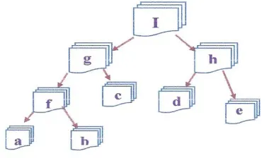
Figure 1. Taxonomic system of subkernels sub-kernels.
Given any two parts of I, denoted by d(a, b), the inertia of the point cloud consisting of points aV and bV with their respective masses ma and mb, is possible to write that the indices of diameter are: (I) = d(g, h), ….., (f) = d(a, b).
In addition, (a) (f) (g) (I). With the above, it is possible to express the inertia In(I) depending on the index diameter of the kernel I index; (I) and their sub-kernels in the following manner:
In(I) = d(g, h) + In(g) +In(h) = N (I) + In(g) +In(h)
That mind a classic decomposition of total inertia In(I) in inertiasinter kernels of the cloud N (I) and the inertia produced by the addition of the inter kernels of g and h; In(g) + In(h). This last also can be expressed as the inertia associated with centers of gravity of the kernels.
Application
Currently, one of the criteria used to assess the functioning of academic and research activities is terminal efficiency, as one of the principal indicators showing the achievements of the corresponding education institution. Since the ESIA, ALM Unit, IPN is has been one of the schools of civil engineering with more students in Mexico, it is very important to know its terminal efficiency, both for licentiate and postgraduate degrees (Casanova, 2010; Casanova, 2012). On the top of the table, the number of graduates for each master’s degree in sciences that is officially known up to 2007, throughout 48 years, is shown. On the bottom of table 1, the terminal efficiency of the master’s degree in civil engineering up to date, which substituted the five previous ones in 2007 is shown. The institution does not update your data automatically, due complicated administrative processes.
The factorial method chosen to describe data under study is the principal component analysis, ACP, since it allows the direct search of simultaneous representation of sets under study I years of graduation and J master degrees in the sciences (Casanova, 2001). The ACP applied on gross data KIJ has the following factorial characteristics:
Table 1. Historical terminal efficiency of master’s degrees in sciences.
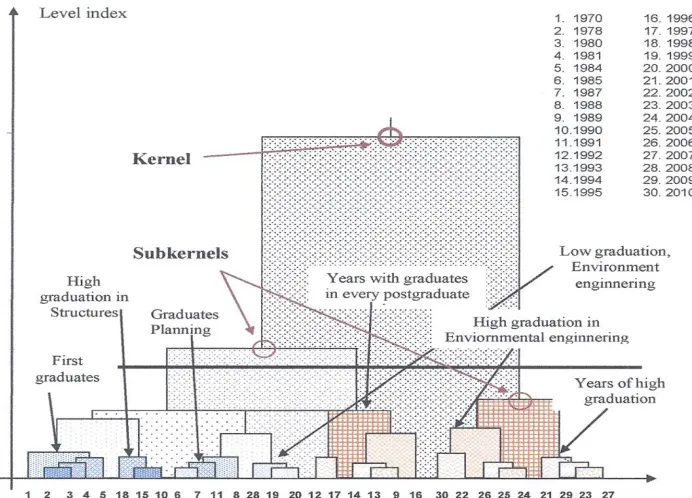
Figure 2, shows the hierarchy of relationship between the years of graduation of master’s degrees in the sciences. Reading and interpretation is based on the value of hierarchical level index, shown on the left of the dendrogram, such being understood as the consecutive order of values from the product of the weight of the class under analysis and its diameter (distance d(i, i´) is the diameter of the smallest part of a hierarchy containing both i and a i´) (Casanova, 2010).
Fig. 2. Hierarchical classification of terminal efficiency of postgraduate degree ESIA IPN, Mexico with hierarchical kernels theory.
Master Degree in Science Number of
graduated students
Period Year of
defense of the first specialty thesis
Terminal efficiency annual index
Structures 58 1962-2010 1970 1.20
Hydraulics 51 1962-2010 1975 1.06
Planning 66 1966-2010 1977 1.37
Soil Mechanics 32 1981-2010 1987 0.66
Environmental Engineering 114 1977-2010 1979 2.37
Doctorate degree
Environmental Hydraulics 5 1998-2010 2000 0.50
Master degree in Engineering
Structures 3 2009-2010 2010 1.5
Hydraulics 5 2009-2010 2010 2.5
Planning 5 2009-2010 2010 2.5
Geotechnics 0 2009-2010 - 0
Conclusions
This work is presented in accordance with its development. The theory developed on hierarchical cores is shown, where the method shown is tributary to three options: i) calculation of distance between elements where factorial coordinates are known; ii) juxtaposition of mass or weight to each element; and iii) calculation of a distance between element classes, depending on an aggregation criterion based on hierarchical cores. From the point of view of the theory developed, it may be seen that from various starting points, the problem of looking for stable classes may be resolved. Starting points may be chosen by the user, with the help of a hierarchical classification. The theorem demonstrated and called Cores Optimal Criterion Theorem allows to implement f and functions from a kth core randomly estimated with the algorithm. In relation to the application of the theory, it is possible to say that the hierarchical dendrogram built is formed by three branches, whose interpretation is absolutely congruent with knowledge on the topic.
Acknowledgement
This document was developed with part of the time devoted to the IPN-SIP 20171058 research project.
References
Benzécri, J P and Benzécri F. (1980). Pratique de L´Analyse des Données. 1. Analyse des Correspondances. Exposé Élémentaire. Dunod. Bordas, Paris. ISBN : 2-04-011227-8.
Casanova del Angel, F. (2001). Análisis multidimensional dedatos. Editorial Logiciels, ISBN: 970-92662-1-7. Mexico. Marion M and Signonello S. (2011). From Histogram Data to Model Data Analysis. B.
Fichet et al (eds.). Classification and Multivariate Analysis for Complex Data Structures, Studies in Classification Data Analysis, and Knowledge Organization. Doi: 10.1007/978-3-642-13312-1_38. Springer- Verlag Berlin Heidelberg.
Diday E and Noirhomme M. (2008). Symbolic Data Analysis and the SODAS software. Wiley. ISBN 978-0-470-01883-5, 457 pages.
Diday E. (2008). Spatial classification. DAM (Discrete Applied Mathematics) Volume 156.
Benzécri J. P, Benzécri F, Bellier L, Bénier B, Blaise S, Bourgarit Ch, Brian, J. P, Cazes P, Dreux Ph, Escofier B, Fénelon J. P, Forcade J, Giudicelli X, Grosmangin A, Guibert B, Hassan A R, Hathout A, Jambu M, Kamal I. H, Kerbaol M, Lacoste A, Lacourt P, Laganier J, Lebesux M O, Lechat J, Le Chappelier M, Lenoir P, Mahé J, Mann C, Marano Ph, Masson M, Moitry J, Müller J, Nakhlé F, Piétri M, M, Richard J F, Rousseau R, Roux G & M, Salem A, Sandor G, Stérpan S, Tabet N, Thauront G, Volle M, Yagolnitzer E y Zloptowicz M. (1976). L´Analyse des Données 1. La Taxinomie. Ed. Dunod Paris. ISBN: 2-04-003316-5. Casanova del Angel, F.
(2010). Structure géométrique des distances hiérarchique No. 41,
pp. 27-47. Revue MODULAD. ISSN: 1769-7387. Casanova del Angel, F. (2012). Terminal Efficiency Analysis of a Postgraduate Degree,