Int. J. IndustrialMathematics (ISSN 2008-5621)
Vol. 8, No. 3, 2016 Article ID IJIM-00823, 14 pages Research Article
Determining Malmquist Productivity Index in DEA and DEA-R
based on Value Efficiency
M. R. Mozaffari ∗†
Received Date: 2015-12-11 Revised Date: 2016-11-09 Accepted Date: 2016-06-11
————————————————————————————————–
Abstract
Malmquist Productivity Index (MPI) is a numeric index that is of great importance in measuring productivity and its changes. In recent years, tools like DEA have been utilized for determining MPI. In the present paper, some models are recommended for calculating MPI when there are just ratio data available. Then, using DEA and DEA-R, some models are proposed under the constant returns to scale (CRS) technology and based on value efficiency (VE) in order to calculate MPI when there is just a ratio of the output to the input data (and vice versa). Finally, in an applied study on 30 welfare service companies under CRS technology, the progress and/or regression of companies are determined in DEA and DEA-R.
Keywords: Malmquist; Value Efficiency; DEA; DEA-R.
—————————————————————————————————–
1
Introduction
D
Eefficiency, utilized for calculating the rela-A is a nonparametric method to evaluate tive efficiency and evaluating the performance of a set of DMUs. This method considers a fron-tier function around the input and output com-ponents. This frontier not only is the most effi-cient units, but also provides an analysis for inef-ficient units. Farrell (1957) for the first time de-termined the efficiency by using a non-parametric method [1]. Data Envelopment Analysis (DEA) was the subject of Rhodes study. The results of his initial research in cooperation with Cooper and Charnes were published in 1978 [2]. By in-troducing the CCR model, Charnes et al. (1978), in fact, extended Farrells idea to multiple inputs and multiple outputs. DEA models are divided∗Corresponding author. [email protected] †Department of Mathematics, Shiraz Branch, Islamic Azad University, Shiraz, Iran.
into two basic groups: input-oriented and output-oriented models. In input-oriented models, in-puts decrease by keeping the status quo for out-puts and in output-oriented models, outout-puts in-crease by keeping the status quo for inputs. Re-turns to scale is a concept that expresses the ratio of inputs to outputs. This ratio can be constant or variable, i.e., it can be increasing or decreas-ing. Banker et al. (1984) introduced models of variable returns to scale [3].
In 1953, Stan Malmquist, a Swedish economist, introduced Malmquist index as an indicator of living standards [4]. Productivity is one of the concepts in studying performance over time. Pro-ductivity index is based on pairwise comparison, which generally refers to the efficiency of an or-ganization over two different periods. To calcu-late efficiency, DEA and Malmquist Index are uti-lized. This index made it possible to divide total productivity into two major components of the change in allocative technological efficiency and
technical efficiency. Then, Caves et al. (1982) uti-lized this index for the first time in the production theory [5]. F¨are et al. (1994) used DEA for cal-culating Malmquist index [6]. Balf et al. (2010) divided this index into two factors of change in the efficiency and technology [7].
Maudos et al. (1999) performed, for the first time, the total factor productivity measurement [8]. Then, Tulkens (1995) paid attention to the non-parametric efficiency in this context [9]. Chen (2003) made use of non-radial Malmquist productivity index for the Chinese industry [10]. Chen and Ali (2004) calculated Malmquist pro-ductivity index by using DEA [11]. Jesus et al. (2005) calculated global Malmquist produc-tivity index with a new viewpoint [12]. Since the evaluation of decision-making units using a com-mon set of weights (CSW) is of great importance, Kao (2010) proposed Malmquist productivity in-dex based on the CSW and conducted an applied research on the data of the Taiwan forests [13]. Wang and Lan (2011) suggested a new method to compute Malmquist productivity index [14].
Along with the dramatic growth of DEA and the focus on the input and output data, the topic of ratio data was introduced. With the integra-tion of DEA and Ratio analysis, Despic et al. (2007) suggested the ratio-based DEA (DEA-R) [15]. Wei et al. (2011) showed the false ineffi-ciency in 21 Taiwan medical centers using DEA-R models [16]. Afterwards, Wei et al. (2011) studied the problems of the CCR model in DEA and the advantages of DEA-R over the previ-ous model [17]. In addition, Wei et al. (2011) computed the efficiency and super-efficiency by developing input-oriented DEA-R models under constant returns to scale technology [18]. Once DEA-R was introduced for ratio data, from a dif-ferent point of view Liu et al. (2011) proposed DEA models without explicit inputs and studied 15 research institutes in China [19]. Mozaffari et al. (2012) studied the relationship between DEA and DEA-R models [20]. Also, Mozaffari et al. (2013) compared cost and revenue efficiency in DEA and DEA-R [21].
Many real problems in organizations can be modeled into a multi-objective program to achieve Pareto-optimal solutions. Pareto-optimal solutions in an organization can be determined with regard to preferences of the decision maker (DM). Korhonen (1986) solved a multiple criteria
problem using interactive methods [22]. In addi-tion, Joro et al. (1998) compared DEA and multi-objective linear programming [23]. At this time, Hamle et al. (1999) suggested a new method in data envelopment analysis by using value ef-ficiency (VE) [24]. Korhonen and Hamle (2000) also raised the subjects of VE with weights re-strictions and later Korhonen et al. (2002) ex-tended the topic so that value efficiency came to the fore [25, 26]. In this regard, Korhonen et al. (2005) and Soleimani-damaneh et al. (2014) studied VE and paid special attention to its ap-plications [27, 28]. Hamle and Korhonen (2013) proposed a new model for benchmarking in het-erogeneous units using value efficiency analysis [29]. Hamle et al. (2014) conducted value effi-ciency analysis of branches of a bank and pro-posed FDH models based on VE [30]. Korhonen et al. meticulously studied the relationship be-tween DEA and VE [31].
In the second section of the article, the basic concepts of MPI and value efficiency are briefly reviewed. In the third section, the MPI model is provided based on VE in DEA. In the fourth sec-tion, first the calculation of MPI in DEA-R is pre-sented, and then the model and relevant theorems are provided. Computing model of MPI based on the VE in DEA-R will also be proposed. In the fifth section, an example is provided in two sub-sections: numerical example and applied study. Finally, some conclusions are stated.
2
Basic concepts
In this section, first a brief review of the efficiency index in DEA is provided. Then, the concept of value efficiency is defined.
2.1 The productivity index in DEA
is no need with this index to have the production cost and product cost data, which are sometimes difficult or impossible to access. It requires no be-havioral assumptions such as profit maximization or cost minimization. Meanwhile, the attractive feature of this index is to decompose the impact of the change in technical efficiency and the im-pact of the change in technological change. The mathematical model of Malmquist productivity index is defined based on the distance function in which the change in total factor productiv-ity between two points of the data is measured by calculating the ratio of the distance of each data point relative to a common technology. Dis-tance Function has many applications in the field of economics, including the fact that it is possi-ble to utilize it to measure and analyze the effi-ciency and productivity. The distance function can be defined and analyzed based on two points: one of them is based on inputs or production fac-tors, as the input-oriented distance function of production that focuses on the minimum use of production factors and the other is based on the output, as the output-oriented distance function that focuses on the maximum production or out-put. The point that should be emphasized is that in the measurement of Malmquist productivity changes index the feature of returns to scale in production is of great significance. Grifell-Tatje. and Lovell (1995) showed that in case that it is as-sumed production technology has variable returns to scale, Malmquist productivity index may not properly measure the changes in total factor pro-ductivity, so it is important in calculation of dis-tance functions and measurement of Malmquist index the assumption of constant returns to scale to be applied [28].
Suppose the jth decision-making unit produces outputs Yjt = (y1tj, ..., ysjt ) with the consumption of inputsXjt= (xt1j, ..., xtmj) at timet. Also, sup-pose the decision-making unit oth produces out-puts Yot+1 = (y1t+1o , ..., ytso+1) with the consump-tion of outputs Xot+1 = (xt1+1o , ..., xtmo+1) at time
t+ 1. Known as output-oriented DEA model un-der CRS technology, model (2.1) evaluates DMUo
at timet+ 1 and other DMUs at time t.
φ∗= M ax φ
s.t ∑nj=1λjxtij+s−i =x t+1
io , ∀i
∑n
j=1λjyrjt −s+r =φytro+1, ∀r
s−i ≥0, s+r ≥0, ∀i,∀r, λj ≥0 ∀i
(2.1) The value of the objective function in model (2.1) for decision-making unit O at timetand for other units at timet+ 1 is represented by the following symbol:
(φ∗)−1=Dto(Xot+1, YOt+1) (2.2)
Therefore, Malmquist productivity index in DEA is calculated by the following equation:
M Do = (
Dt
o(Xot+1, YOt+1)Dot+1(Xot+1, YOt+1)
Dt
o(Xot, YOt)D t+1
o (Xot, YOt)
)1/2
(2.3) In linear programming model (2.1) the value of
φ∗ can be calculated in the first phase and then in the second phase the maximum value of slack variables (s−i , s+r) can be calculated. Units in model (2.1) are called efficient if φ∗ = 1 in the first phase and all optimal solutions of slack vari-ables be zero, i.e. (s−i ∗, s+r∗) = (o, o), in the sec-ond phase.
2.2 Value Efficiency (VE)
In this section, initial definitions of cone and the cone of feasible directions are provided and then the value efficiency model is defined and pre-sented.
Definition 2.1 A nonempty set defined in an n-dimensional Euclidean space Rn is called a cone with vertex x, if x +y ∈ GX ⇒ x+λy ∈ GX
for all Rn. The cone with the origin as vertex is denoted by G. Note that vertex. A singleton {x} is also a cone with vertex x.
Definition 2.2 Let X is a nonempty polytope in Rn and letx∈X. The cone D(x) inRnis called the cone of feasible directions of X at x, ifD(x) =
{d|x +λd ∈ X, f or allλ ∈ (0, δ)f or δ > 0}. Each d∈D(x), d̸= 0, is called a feasible di-rection. The cone GX ={y|y=x+d, d∈D(x)}
is called the tangent cone of X at x and the cone WX ={s|s=y+z, z∈Rn} the augmented
In general, the output-oriented technical effi-ciency of the decision-making units in DEA is equal to the ratio of the output of the unit under analysis to the output obtained by stretching the radial line which passes through the origin and cuts the DEA frontier. However, in computing the technical efficiency in DEA units called MPS do not play any role, though it is the manager that determines MPS and uses it in the analy-sis. Of course, VE enjoys problems such as using the approximate function of VE. But due to the use of manager views for the introduction of MPS and taking into account the managers idea in the analysis of the efficiency and also measuring the distance difference with MPSs, VE can be used following DEA models. VE scale can be easily calculated and it is required to display MPS as non-negative linear combination (with the condi-tion of constant returns to scale) of units that are on DEA efficiency frontier. Khorhoneh proposed the output-oriented DEA model for calculating value efficiency (VE) under CRS as follows:
M ax σ
s.t ∑∑jn=1λjxij +si−=xio, ∀i n
j=1λjyrj−σyro−s+r =yro,∀r
s−i ≥0, s+r ≥0, ∀i,∀r,
λj :
{
≥0 if λ∗j = 0 =f ree if λ∗j >0
(2.4)
In model (2.4) λ∗j is calculated from the equa-tion (X∗, Y∗) = (∑j∈M P Sλ∗jxij,
∑
j∈M P Sλ∗jyrj). In addition, (X∗, Y∗) is located on the CRS fron-tier.
Definition 2.3 DMU0 is called value efficiency if in model (2.4) σ∗ = 0 and in all opti-mal solutions the slack variables are zero, i.e.
(s−∗i , s+r∗) = (o, o).
3
MPI based on VE in DEA
To calculate the output-oriented Malmquist Pro-ductivity Index (MPI) under CRS technology the following model is proposed based on the effi-ciency value:
α∗= M ax α
s.t ∑∑nj=1λjxtij+si =xtio+1, ∀i n
j=1λjyrjt −αyrot+1−sr =ytro+1,∀r
si≥0, sr≥0, ∀i,∀r,
λj :
{
≥0 if λ∗j = 0 =f ree if λ∗j >0
(3.5) The value of objective function (3.5) for decision-making unit o at time t+ 1 and in case that other units are at time t is represented by the symbol below:
(1 +α∗)−1 =Eot(Xot+1, YOt+1) (3.6)
The efficiency index in DEA is calculated based on the value efficiency from the following equa-tion:
M Eo= (
Eot(Xot+1, YOt+1)Eot+1(Xot+1, YOt+1)
Et
o(Xot, YOt)E t+1
o (Xot, YOt)
)1/2
(3.7) In general, in DEA the scale efficiency is cal-culated from basic input- and/or output-oriented DEA models without the taking into account the manager’s idea in the analysis. But in models proposed Joro et al. [27] the value efficiency is calculated based on the MPS and the manager’s idea. The difference model (2.1) and (3.5) is only in determining the variable symbol ofλj.
4
Computing
MPI
for
ratio
data
In this section, first computing models of MPI in DEA-R and then computing models of MPI based on VE in DEA-R are suggested.
4.1 MPI in DEA-R
Suppose jth decision-making unit with the con-sumption of inputs, Xjt = (xt1j, ..., xtmj), at time
t produces outputs, Yjt = (y1tj, ..., ysjt ), at timet. Suppose also that the ratio of output to input are defined at two successive times tand t+ 1.
M ax θ
s.t ∑nj=1µj( yt
rj xt
ij)−θ( ytro+1 xtio+1)−sir = (ytro+1
xtio+1) ∀i,∀r,
∑n
j=1µj = 1,
sir≥0, ∀i,∀r,
µj ≥0, ∀j.
Model (4.8) is a linear programming problem in-troduced as the output-oriented DEA-R for the evaluation of DMUo at timet+ 1 when the other units are at time t+ 1 [15, 16]. Using optimal model (4.8), we have:
(θ∗)−1 =Hot(Xot+1, YOt+1) (4.9)
Malmquist Productivity Index (MPI) in DEA-R is obtained.by equation (4.10)
M Ho= (
Ht
o(Xot+1, YOt+1)Hot+1(Xot+1, YOt+1)
Ht
o(Xot, YOt)H t+1
o (Xot, YOt)
)1/2
(4.10) In this section, theorems that states the rela-tionship among the proposed models in the DEA and DEA-R in order to calculate Malmquist Pro-ductivity Index are provided.
Theorem 4.1 In models (2.1) and (4.8) in case of one input and s output there is Hot(Xot+1, YOt+1) = Dot(Xot+1, YOt+1) (the scale ef-ficiency obtained from models (2.1) and (4.8) in case of one input and s output are equal.)
Proof. Consider the output-oriented multiplier model under constant returns to scale technology for evaluating DM Uo in DEA as following.
M in ∑mi=1vixio
s.t ∑sr=1uryrj−
∑m
i=1vixij ≤0 ∀j,
∑s
r=1uryro = 1,
vi≥0 ur≥0, ∀i,∀r.
(4.11) In addition, consider the output-oriented model in multiplier form with constant returns to scale technology for analyzing DEA-R as follows [17].
M in θ
s.t ∑mi=1∑sr=1wir( yrj xij yro xio ) ∑m i=1 ∑s
r=1wir= 1,
sir ≥0, ∀i,∀r.
(4.12)
Without any change in the generality of the argument, assume there is one input and
s outputs. So, considering the value of the objective function as θ, we have v1x1o = θ, then v1 = xθ1o. Also, with defining ur = y1rpw1r
we have ∑sr=1uryrp =
∑s r=1
1
yrpw1r(yrp) = 1. Furthermore, with the placement of v1 and ur in the provision∑sr=1uryrj−
∑m
i=1vixij ≤0 we have:
∑s r=1
1
yrow1ryrj− θ
x1oxij ≤0
=⇒ ∑sr=1y1
row1ryrj ≤ θ x1oxij
=⇒ ∑sr=1wir yrj xij yro xio ≤
θ
If we consider DM Uo at time t + 1 and
DM Uj j ̸= 0 at time t, model (4.11) is the dual model (2.1) and also model (4.12) is the dual model (4.8) in case of one input and s outputs. So the optimal values of models (2.1) and (4.8) are equal.
Theorem 4.2 In models 2 and 9 in case of m inputs and s outputs, we have:
Hot(Xot+1, YOt+1)≤Dot(Xot+1, YOt+1)
Proof. For evaluating, the DM Uo output-oriented DEA multiplier model under CRS tech-nology taken from the idea of Despic et al. [15] is presented as below:
φ∗DEA =M in(u,v) M axj
∑s
r=1ur(yyrjro)
∑m
i=1vi(
xij xio) s
∑
r=1
ur= 1, m
∑
i=1
vi = 1
ur≥0, vi≥0. i= 1, .., m, r= 1, .., s. (4.13)
Harmonic efficiency models for evaluatingDM Uo based on the idea of Wei et al. [16] is presented as follows.
φ∗H−DEA−R=
M in(u,v)M axj( s
∑
r=1
ur(
yrj yro )).( m ∑ i=1
vi(
xij xio )) s ∑ r=1
ur = 1, m
∑
i=1
vi= 1
ur ≥0, vi ≥0. i= 1, .., m, r = 1, .., s.
(4.14)
In models (4.13) and (4.14) definitions of are considered and applied. By multiplying model
(4.13) in the expression ∑m
i=1vi(1/Xij′ ) ∑m
i=1vi(1/Xij′ ) we have:
M in(u,v) M axj ∑s
r=1ur(Yrj′) ∑m
i=1vi(Xij′ ) × ∑m
i=1vi(1/Xij′ ) ∑m
i=1vi(1/Xij′ ); therefore, using the equation ∑mi=1vi(Xij′ ) ×
∑m
models (4.13) and (4.14) can be obtained as fol-lows.
φ∗DEA
=M in(u,v)M axj
∑s
r=1ur(Yrj′ )
∑m
i=1vi(Xij′ )
×
∑m
i=1vi(1/Xij′ )
∑m
i=1vi(1/Xij′ )
≤M in(u,v)M axj s
∑
r=1
ur(Yrj′ ). m
∑
i=1
vi(1/Xij′ )
φ∗DEA≤φ∗H−DEA−R
=⇒ 1
φ∗DEA ≥
1
φ∗H−DEA−R
This means:
Now, considering DM Uo at time t + 1 and
DM Uj j ̸= 0 at time t and model (4.13) is equal to thedual model (2.1)and model (4.14) is equal to dual model (4.8), so
Hot(Xot+1, YOt+1)≤Dto(Xot+1, YOt+1)
4.2 MPI based on the VE in DEA-R
In this section, first the output-oriented DEA-R models based on the value efficiency in CRS tech-nology is recommended to calculate MPI. The re-lated theorems to the proposed models are then provided. Therefore, considering DM Uo at time
t + 1 and DM Uj such that j ̸= 0 at time t, the value efficiency models in the output-oriented DEA-R are proposed as following:
M ax β
n
∑
j=1
µj(
ytrj
xtij)−β( yrot+1
xtio+1)−sir= ( yrot+1 xtio+1)
s.t
µj :
{
≥0 if µ∗j = 0 =f ree if µ∗j >0 n
∑
j=1
µj = 1, sir ≥0,
(4.15)
In model (4.15) the optimal value is calculated from the equation
∑
j∈M P S
µ∗j = 1, (X∗, Y∗)
= ( ∑
j∈M P S
µ∗jxij,
∑
j∈M P S
µ∗jyrj).
The productivity index in DEA-R based on the value efficiency is calculated from the following equation.
(1 +β∗)−1 =Rto(Xot+1, YOt+1) (4.16)
M Ro = (
Rto(Xot+1, YOt+1)Rto+1(Xot+1, YOt+1)
Rt
o(Xot, YOt)R t+1
o (Xot, YOt)
)1/2
(4.17)
In GAMS program constraints of model (4.15) with the separation of free variables in symbols and nonnegative variables is as follows.
Equations
Objective, Con1(i, r), Con2;
Objective.. z=e=T eta;
Con1(i, r)..
Sum(j,(y1(j, r)/x1(j, i))∗Lambda(j))
+Sum(p,(y1p(p, r)/x1p(p, i))∗mu(p))
−T eta∗(y2o(r)/x2o(i))−s(i, r) =e=y2o(r)/x2o(i);
Con2..
Sum(j, Lambda(j))
+Sum(p, mu(p)) =e= 1;
F ileResults/Results.txt/;
M odele M odel/All/;
The reason of proposing model (4.15) based on the ideas of Korhonen is presented as follows [27].
Lemma 4.1 Let Λ = {µ =
(µ1, ..., µn)|
∑n
j=1µj = 1, µj ≥ 0 j = 1, ..., n}
be a nonempty polytope and µo ∈Λ an arbitrary point. Then Gµo = ΛO,
ΛO = {(µ1, ..., µn)|
∑n
j=1µj = 1, µj ≥ 0 if µoj = 0, and otherwise µoj is f ree, j= 1, ..., n}
Proof. Clearly the tangent cone of an affine set Λa = {(µ1, ..., µn)|
∑n
j=1µj = 1} at µo is
Λa itself. Moreover, the tangent cone of the closed half-space Hj = {µ = (µ1, ..., µn)| µj ≥ 0 j = 1, ..., n} at µo is Rn, if µoj >0 and Hj if
Lemma 4.2 Let TR = {yx|
∑n
j=1µj(yxrjij) = y
x, µ ∈ Λ} where, Λ = {(µ1, ..., µn)|
∑n
j=1µj =
1, µj ≥ 0 j = 1, ..., n}, be a linear
transformation of a nonempty polytope Λ and
(yo
xo) ∈ TR an arbitrary point. Let µ
0 ∈
Λ be any point such that ∑nj=1µoj(yrj xij) = yo
xo. Then the tangent cone of TR at ( yo xo) is
G(yo xo)=
∑n j=1µoj(
yrj xij)={
y x|
y x=
∑n
j=1µj(yrjxij),µ∈Gµo}.
Proof. Any µ ∈ Gµo,y x ̸=
yo
xo, defines a fea-sible direction (yx − yo
xo) for TR at ( yo
xo), which must be generated by a feasible direction (µ−µo) for Λ at µo. Thus Gyo
xo ⊂ (
∑n j=1µj(
yrj xij))Gµ
o.
Any µ ∈ Gµo,(µ ̸= µo) defines a feasible direc-tion (µ−µo) for Λ at µo, which defines a fea-sible direction (xy − yo
xo) for TR at ( yo
xo). Thus
Gyo xo ⊃(
∑n j=1µj(
yrj xij))Gµo.
Theorem 4.3 Wu∗ is the largest cone with
the property Wu∗ ⊂ V = {u|v(u) ≤
v(u∗), f or any v∈E(u∗)}.
Proof. See [27] Let u∗ = [yx∗∗]∈ TR be the DMs most preferred solution. Then u∗ ∈ TR, an ar-bitrary point in the input/output space, is value inefficient with respect to any strictly increasing pseudoconcave value function v(u), u= [yx] with a maximum at pointu∗, if the optimum valueZ∗
of the following problem is strictly positive:
M ax Z =θ
s.t ∑nj=1µj(yxrjij)−θ(yxroio)−sir = (yro
xio) ∀i,∀r,
∑n
j=1µj = 1,
sir ≥0, ∀i,∀r,
(4.18)
Where µ∗ ∈Λ correspond to the most preferred solutions, yx =∑nj=1µ∗j(yrj
xij).
Proof. By Lemmas 4.1 and 4.2 the tangent cone of TR at u∗ is the set where TR = {yx|u =
∑n j=1µj(
yri xij) =
y
x, µ ∈ Λ}, where the tangent cone of Λ at µ∗ is Gµ∗ ={(µ1, ..., µn)|
∑n
j=1µj = 1, µj ≥0if µ∗j = 0, and otherwise µ∗j is f ree, j= 1, ..., n}. The augmented tangent cone Wu∗ of T atu∗ is the set{yx|yx =∑nj=1µj(yxrjij) +dxy, dxy ≤ 0 , µ ∈ Λ}. Therefore (8) hasa solution with
θ ≥0 only if [xy] ∈Wu∗. Now let (Z∗, θs, µs) be a solution of (4.8). With ε > 0, Z8 > 0 only if either θs >0 or θs = 0 and (sir) ̸= 0. In either case, [yxss] ∈ Wu∗ and y
s
xs =
∑n j=1µsj(
yrj xij) ≥
y x and yxss ̸= yx. Thus v(yx)≤v(y
s
xs)≤v(y
∗
x∗), and by Theorem4.1, (y,x) is value inefficient.
Definition 4.1 The (weighted) value efficiency score for point uo = [yo
xo] is defined as Where θ s
is the value ofθat the optimal solution of problem (4.18).
Therefore, model (4.15) is of great significance in calculating MPI when the ratio data of the output to input is available.
5
Numerical Example
In this section, first five decision-making units are considered in the numerical example for calculat-ing MPI in DEA and DEA-R. Then an applied study on 30 welfare companies is provided in or-der to compare Malmquist productivity index in DEA and DEA-R.
5.1 Numerical Example
In this section, five decision-making units with two outputs (o1 and o2) and one input (I1) are considered in calculating Malmquist productivity index in DEA and DEA-R and the efficiency is treated based on the value efficiency. Figure 1 shows the CRS production possibility set of five decision-making units at two times of tand t+ 1 with two outputs and one input. All units at timetand t+ 1 are on the efficiency frontier and are compared using Malmquist efficiency index in the table below. Dashed line shows the frontier of five decision-making units (D1, A1, B1, C1, E1) at time t and solid line displays the frontier of five decision-making units (D2, A2, B2, C2, E2) at time t+ 1. In Table 2, the second up to fifth
Figure 1: The production possibility set at time t andt+ 1.
Table 1: Input and Output data at timetandt+ 1
DMU I1 O1 O2 DMU I1 O1 O2
A A1 1 4 8 A2 1 6 6.8
B B1 1 6 6.8 B2 1 10 6.8
C C1 1 9 5 C2 1 11 5
D D1 1 2 8 D2 1 2 6.8
E E1 1 9 3 E2 1 11 3
Table 2: The value efficiency and the value of MPI at timest andt+ 1
DMU D11 D22 D21 D12 MD=MH
ALL DMU
A 1 1 1.1765 1 0.921943
-B 1 1 1 1.2308 1.109414 +
C 1 1 0.8548 1.2222 1.195746 +
D 1 1 1.1765 0.85 0.849989
-E 1 1 0.8182 1.2222 1.222198 +
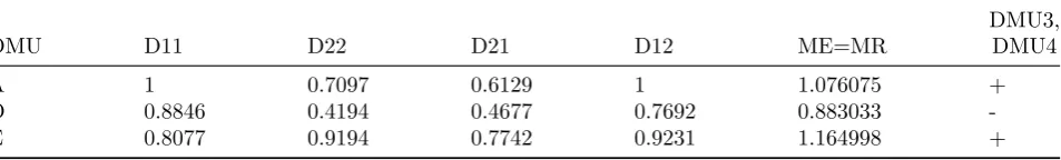
Table 3: The value of MPI based on the scale efficiency at timestandt+ 1 (units B and C are MPS)
DMU D11 D22 D21 D12 ME=MR
DMU3, DMU4
A 1 0.7097 0.6129 1 1.076075 +
D 0.8846 0.4194 0.4677 0.7692 0.883033
-E 0.8077 0.9194 0.7742 0.9231 1.164998 +
of MPI in DEA and DEA-R, i.e. models (2.3) and (4.10). According to Theorem 4.1, since in the example there are multiple inputs and one output, it is observed that the efficiency and value of MPI obtained by equations (2.3) and (4.10) are exactly equal. Overall, units B, C and E show progress at sequential times t and t+ 1, while units D and A show regression at same times. In Table3, with considering units B and C as MPS by the manager, Malmquist productivity index was compared based on VE in DEA and DEA-R. Unit A is compared with MPS units, i.e. B and C. Therefore, the second output of unit A1 which is 8 compared to the second output of unit B1 which is 6.8 showed an increase, and similarly at time
t+ 1 the second output of unit A2 which is 6.8 is constant compared to the second output of unit B2 which is 6.8. Generally, the results of models of unit A showed a progress considering MPS of B and C. Of course, the mount of progress in unit A is less than unit E, as shown in Table3below. Similarly, with MPI value equal to 0.883033 unit D had a regression at two consecutive times.
5.2 Applied Study
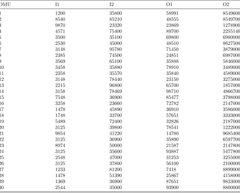
In this section, 30 welfare companies, which pro-vide retirees with utilities such as seasonal out-ings, meals and holding special celebrations are to be analyzed. In Table 4, input and output data related the second quarter of 2014 and 2015 are presented. The government has a plan to evalu-ate the productivity index of all companies dur-ing two consecutive periods. The problem is that many companies do not provide real data of their current liability, current cost and asset as well as total assets for the government.
Table 4: Input and output data related to the second quarter of 2014
DMU I1 I2 O1 O2
1 1200 35800 58991 8549600
2 8540 85210 48555 8549700
3 9870 23320 23869 1278900
4 4571 75400 89700 2255140
5 3500 35100 69800 6980000
6 2530 45000 48510 8627500
7 3148 95780 71450 3879000
8 2385 74500 24851 6987000
9 3569 65100 35888 5846000
10 3458 35880 78910 3489000
11 2358 35570 35840 4589000
12 3148 78440 23150 3275000
13 2215 96800 65700 1857000
14 3158 78469 98710 4866700
15 7548 36900 85477 3798000
16 3258 23660 72782 2147000
17 1478 45890 36910 3586000
18 1748 33700 57651 3333000
19 5489 72400 32826 2187000
20 3125 39800 78541 1222000
21 9854 41220 14780 9685400
22 3125 36900 35890 6597700
23 8974 50000 21587 2147800
24 3125 35600 93887 5477800
25 2548 47000 31253 3255000
26 3125 37800 56100 2100000
27 1233 81200 7418 8899000
28 1478 51390 25867 4158000
29 1369 36900 87651 9833000
30 2544 35000 93900 8800000
second input I2 is related to the cost of the com-pany. Current liabilities include bank overdrafts, taxes and other obligations that are reasonably expected to be. The first output O1 is related to current assets the and second output O2 is related to total assets in US Dollars. Current assets consisted of cash, temporary investments, and prepaid expenses.
However, from the viewpoint of government wel-fare companies are required to provide financial guarantees and have sufficient experience in pro-viding related services. As observed in this study, the companies under study first refused to pro-vide the related input and output data defined in the previous sections as they tried to show the best of their companies. This means that they only provided the ratio data, i.e. the ratio of out-put data to inout-put data; though, the government obtained the necessary data with inspection and using backup data. Therefore, in order to
calcu-late the Malmquist productivity index, we con-sider two viewpoints.
A) Input and output data are available
At the end of 2014 and 2015, the government is able to collect data by making quarterly backups and using online data, although problems such as the malfunction of data transmission systems or the change of evaluation criteria for companies (inputs and outputs) still exist in this regard.
B) A ratio of output data to input data is available
This is the case when the government requires the input and output data from companies, but they just provide a ratio of output data to input data. In this case, the ratio data are as follows:
The ratio OI11 is the ratio of companies current assets to the current liability, which is defined as quick ratio.
Table 5: Input and Output Data of the Second Quarter of 2015
DMU I1 I2 O1 O2
1 1200 35800 58991 8549600
2 8540 85210 48555 8549700
3 9870 23320 23869 1278900
4 4571 75400 89700 2255140
5 3500 35100 69800 6980000
6 2530 45000 48510 8627500
7 3148 95780 71450 3879000
8 2385 74500 24851 6987000
9 3569 65100 35888 5846000
10 3458 35880 78910 3489000
11 2358 35570 35840 4589000
12 3148 78440 23150 3275000
13 2215 96800 65700 1857000
14 3158 78469 98710 4866700
15 7548 36900 85477 3798000
16 3258 23660 72782 2147000
17 1478 45890 36910 3586000
18 1748 33700 57651 3333000
19 5489 72400 32826 2187000
20 3125 39800 78541 1222000
21 9854 41220 14780 9685400
22 3125 36900 35890 6597700
23 8974 50000 21587 2147800
24 3125 35600 93887 5477800
25 2548 47000 31253 3255000
26 3125 37800 56100 2100000
27 1233 81200 7418 8899000
28 1478 51390 25867 4158000
29 1369 36900 87651 9833000
30 2544 35000 93900 8800000
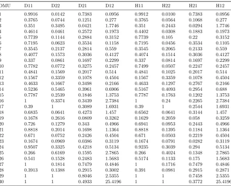
to which a company can continue to operate. In Table 6, the efficiency scores of model (2.2) and model (4.9) are presented in the second to fifth columns and in the sixth to ninth columns, respectively. According to Theorem 4.2, as the applied study is based on two inputs and two out-puts, it is observed that the efficiency scores of model (2.2) are greater than or equal to those of model (10).
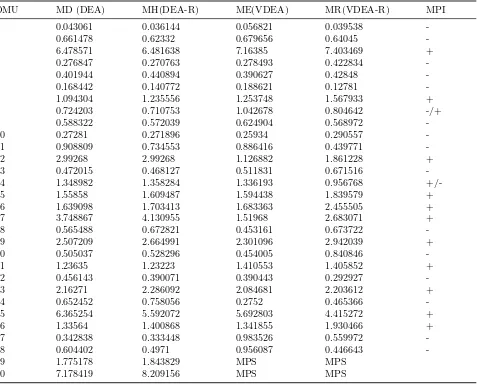
The managers determined a combination of units 29 and 30 as the MPS. Accordingly, Malmquist productivity index is presented based on DEA and DEA-R in Table7. Considering the extensive experience of companies 29 and 30 in providing welfare services, the manager insists on calculat-ing their efficiencies and then Malmquist produc-tivity index. When the input and output data are available, Malmquist productivity index can be calculated by models (2.3) and (3.7). How-ever, if only the ratio of output data to input
data is available, Malmquist productivity index can be calculated by models (4.10) and (4.17). Using management viewpoints, computing tech-nical efficiency and Malmquist productivity index according to management viewpoints, and apply-ing the managers views are of great importance as a tool in discussing value efficiency analysis and DEA [27].
In Table7, a combination of units 29 and 30 is the MPS. In addition, the values obtained by the four models (2.3), (4.10), (3.7), and (4.17) are repre-sented by DEA, DEA-R, VDEA and VDEA-R, respectively, in the second to fifth columns of Ta-ble 7.
Table 6: The scale efficiencies of DEA and DEA-R in 2014 and 2015 (solutions of Model 2 and 9)
DMU D11 D22 D21 D12 H11 H22 H21 H12
1 0.9916 0.0142 0.7383 0.0956 0.9912 0.0100 0.7383 0.0956 2 0.3765 0.0744 0.1251 0.277 0.3765 0.0564 0.1068 0.277 3 0.351 0.3495 0.0421 1.7746 0.351 0.2443 0.0294 1.7746 4 0.4614 0.0461 0.2572 0.1973 0.4402 0.0308 0.1883 0.1973 5 0.7739 0.1144 0.2884 0.3152 0.7739 0.105 0.22 0.3152 6 0.7195 0.0623 0.3534 0.1158 0.7195 0.0456 0.3534 0.1105 7 0.3545 0.2137 0.2814 0.559 0.3545 0.2065 0.2133 0.559 8 0.4077 0.1573 0.3036 0.4127 0.4074 0.1514 0.3036 0.4127 9 0.337 0.0861 0.1697 0.2299 0.337 0.0814 0.1697 0.2299 10 0.7782 0.0772 0.3275 0.2457 0.7499 0.0507 0.2247 0.2457 11 0.4841 0.1569 0.2017 0.514 0.4841 0.1025 0.2017 0.514 12 0.1567 0.3359 0.1078 0.4504 0.1567 0.3359 0.1078 0.4504 13 0.4633 0.1667 0.3498 0.2166 0.4633 0.1297 0.2767 0.2166 14 0.5236 0.5465 0.3961 0.6906 0.5167 0.4093 0.2954 0.688 15 0.7787 0.2539 0.1846 1.3753 0.7787 0.1763 0.1202 1.3753
16 1 0.3374 0.3439 2.7384 1 0.24 0.2265 2.7384
17 0.39 1 0.3089 1.6931 0.39 1 0.2544 1.6931
18 0.6835 0.0641 0.4273 1.457 0.6562 0.0641 0.3144 1.457 19 0.1678 0.2616 0.0809 0.3262 0.1629 0.2059 0.058 0.3259 20 0.726 0.1279 0.343 0.4966 0.6941 0.0953 0.2443 0.4966 21 0.8818 0.2014 0.1698 1.1364 0.8818 0.1395 0.1184 1.1364 22 0.671 0.0752 0.2426 0.4504 0.671 0.0503 0.2219 0.4504 23 0.1674 0.0969 0.0386 0.3119 0.1674 0.0791 0.0282 0.3119 24 0.9507 0.3325 0.4218 0.5134 0.9235 0.3039 0.294 0.5134 25 0.266 0.6169 0.1595 2.7865 0.266 0.4024 0.1348 2.7865 26 0.541 0.1528 0.2483 1.5683 0.5174 0.1133 0.175 1.5683
27 1 0.1814 0.7479 0.4846 1 0.1716 0.7479 0.4846
28 0.3913 0.1388 0.2915 0.3002 0.391 0.0981 0.2915 0.2871
29 1 1 0.8046 2.5355 1 1 0.7458 2.5355
30 1 1 0.4933 25.4196 1 1 0.3772 25.4196
8 and 14 have progressed in VDEA and regressed in VDEA-R.
DEA and DEA-R models based on the value ef-ficiency are models (3.7) and (4.17), respectively, and their results are shown in Table 7. Compa-nies 1 and 6 enjoy the lowest values of output-oriented Malmquist productivity index and show the highest regression. Companies 3 and 30 enjoy the highest values of output-oriented Malmquist productivity index and show the highest progress. Similarly, in DEA-R based on the vale efficiency, there are Max and Min values in Malmquist pro-ductivity index for the aforementioned companies and they present similar behaviors in DEA and DEA-R models.
Companies 3, 7, 12, 14, 15, 16, 17, 19, 21, 23, 25, 29 and 30 have increasing MPI index in DEA and DEA-R. If based on VE the MPI index is considered in DEA and DEA-R, the difference of columns are 1.042678 and 0.804642 Unit 8 have
a progress in VDEA, i.e. it shows progress com-paring with MPSs; though, it shows regression in the normal sate. Unit 12 in VDEA and VDEA-R have less progress in comparison to the normal state, i.e. the selecting MPS for unit 12 is not appropriate. However, compared to the normal state unit 16 shows more progress in VDEA and VDEA-R, i.e. selecting MPS for 16 units is suit-able. Overall, the highest progress in VDEA is related to units 3 and 25, respectively and the highest regression in VDEA is related to unit 1 and 6, respectively. Similar behavior was noted for VDEA-R.
Sim-Table 7: MPI values in DEA, DEA-R, VDEA, and VDEA-R in 2014 and 2015.
DMU MD (DEA) MH(DEA-R) ME(VDEA) MR(VDEA-R) MPI
1 0.043061 0.036144 0.056821 0.039538
-2 0.661478 0.62332 0.679656 0.64045
-3 6.478571 6.481638 7.16385 7.403469 +
4 0.276847 0.270763 0.278493 0.422834
-5 0.401944 0.440894 0.390627 0.42848
-6 0.168442 0.140772 0.188621 0.12781
-7 1.094304 1.235556 1.253748 1.567933 +
8 0.724203 0.710753 1.042678 0.804642 -/+
9 0.588322 0.572039 0.624904 0.568972
-10 0.27281 0.271896 0.25934 0.290557
-11 0.908809 0.734553 0.886416 0.439771
-12 2.99268 2.99268 1.126882 1.861228 +
13 0.472015 0.468127 0.511831 0.671516
-14 1.348982 1.358284 1.336193 0.956768
+/-15 1.55858 1.609487 1.594438 1.839579 +
16 1.639098 1.703413 1.683363 2.455505 +
17 3.748867 4.130955 1.51968 2.683071 +
18 0.565488 0.672821 0.453161 0.673722
-19 2.507209 2.664991 2.301096 2.942039 +
20 0.505037 0.528296 0.454005 0.840846
-21 1.23635 1.23223 1.410553 1.405852 +
22 0.456143 0.390071 0.390443 0.292927
-23 2.16271 2.286092 2.084681 2.203612 +
24 0.652452 0.758056 0.2752 0.465366
-25 6.365254 5.592072 5.692803 4.415272 +
26 1.33564 1.400868 1.341855 1.930466 +
27 0.342838 0.333448 0.983526 0.559972
-28 0.604402 0.4971 0.956087 0.446643
-29 1.775178 1.843829 MPS MPS
30 7.178419 8.209156 MPS MPS
ilarly, units 29 and 30 are considered as MPS, units 3 and 25 as units with the highest progress and units 1 and 6 as units with the greatest re-gressions in both VDEA and VDEA-R.
6
Conclusion
In DEA when data are ratio the scale efficiencies and then MPI cannot easily be identified. With using DEA-R it is possible to find MPI for ra-tio data beside problems such as (input-oriented) false-inefficiency using ε as a non-Archimedean number which leads to weight restrictions in DEA. The relationship between MPI in DEA and DEA-R and classification of units in this evalua-tion is very important. In this paper, in addievalua-tion to calculating MPI in DEA and DEA-R the dis-cussion of VE analysis has also been used. With introducing units as MPS, VE applies some crite-ria according to the management viewpoints that
References
[1] M. J. Farrell, The measurement of produc-tivity efficiency, Journal of The Royal Sta-tistical Society Series A: General 120 (1957) 253-281.
[2] A. Charnes, W. W. Cooper, E. Rhodes,
Measuring the efficiency of decision making units, European Journal of Operational Re-search 2 (1978) 429-444.
[3] R. D.Banker, A. Charnes, W. W. Cooper,
Some models estimating technical and scale inefficiencies in data envelopment analysis, Management Science 30 (1984) 1078-1092.
[4] S. Malmquist, Index numbers and indif-ference surfaces, Trabajos de Estatistica 4 (1953) 209-242.
[5] W. D. Caves, L. R. Christensen, W. E. Diew-ert, The economic theory of index numbers and the measurement of input, output, and savings banks, European Economic Review 40 (1982) 1281-1303.
[6] R. F¨are, S. Grosskopf, M. Norris, Z. Zhang,
Productivity growth, technical progress and efficiency change in industrialized countries, American Economic Review 84 (1994) 66-83.
[7] F. R. Balf, F. Hosseinzadeh Lotfi, M. Al-izadeh Afrouzi, The interval malmquist pro-ductivity index in DEA, Iranian Journal of Optimization 2 (2010) 311-322.
[8] J. Maudos, J. M. Pastor, L. Serrano, Total factor productivity measurement and human capital in OECD countries, Economics Let-ters (1999).
[9] H. Tulkens, P. VandenEeckaut, Non-parametric efficiency, progress and regress measures for panel data: Methodological as-pects, European Journal of Operational Re-search 80 (1995) 474-499.
[10] Y. Chen, A non-radial. Malmquist produc-tivity index with an illustrative application to Chinese major industries, International Journal of Production Economics 83 (2003) 27-35.
[11] Y. Chen, A. I. Ali, DEA Malmquist produc-tivity measure: new insights with an applica-tion to computer industry, European Journal of Operational Research 159 (2004) 239-249.
[12] T. Jesus, C. A. Pastor Knox Lovell, A global MalmquistProductivity Index, Eco-nomics Letters 88 (2005) 266-271.
[13] C. Kao, Malmquist productivity index based on common-weights DEA: The case of Tai-wan forests after reorganization, Omega 38 (2010) 484-491.
[14] Y. M. Wang, Y. X. Lan, Measuring malmquist productivity index: A new ap-proach based on double frontiers data en-velopment analysis,Mathematical and Com-puter Modelling54 (2011) 2760-2771. [15] O. Despic, M. Despic, J. C. Paradi,DEA-R:
Ratio-based comparative efficiency model, its mathematical relation to DEA and its use in applications, Journal of Productivity Analy-sis 28 (2007) 33-44.
[16] C. K. Wei, L. C. Chen, R. K. Li, C. H. Tsai,
Using the DEA-R model in the hospital in-dustry to study the pseudo-inefficiency prob-lem, Expert Systems with Applications 38 (2011) 2172-2176.
[17] C. K. Wei, L. C. Chen, R. K. Li, C. H. Tsai,
Exploration of efficiency underestimation of CCR model: Based on medical sectors with DEA-R model, Expert Systems with Appli-cations 38 (2011) 3155-3160.
[18] C. K. Wei, L. C. Chen, R. K. Li, C. H. Tsai,
A study of developing an input- oriented ratio-based comparative efficiency model, Ex-pert Systems with Applications 38 (2011) 2473-2477.
[19] W. B. Liu, D. Q. Zhang, W. Meng, X. X. Li, F. Xu, A study of DEA models without explicit inputs, Omega 39 (2011) 472-480.
[20] M. R. Mozaffari, J. Gerami, J. Jablonsky,
[21] M. R. Mozaffari, P. Kamyab, J. Jablonsky , J. Gerami, Cost and revenue efficiency in DEA-R models, Computers & Industrial En-gineering 78 (2014) 188-194.
[22] P. Korhonen, J. Laakso,A visual interactive method for solving the multiple criteria prob-lem, European Journal of Operational Re-search 24 (1986) 277-287.
[23] T. Joro, P. Korhonen, J. Wallenius, Struc-tural comparison of data envelopment anal-ysis and multiple objective linear program-ming, Management Science 44 (1986) 962-970.
[24] M. Halme, T. Joro, P. Korhonen, S. Salo, J. Wallenius, A value efficiency approach to incorporating preference information in data envelopment analysis, Management Science 45 (1999) 103-115.
[25] M. Halme, P. Korhonen,Restricting weights in value efficiency analysis, European Jour-nal of OperatioJour-nal Research 126 (2000) 175-188.
[26] P. Korhonen, A. Siljam¨aki , M. Soismaa,On the use of value efficiency analysis and fur-ther developments, Journal of Productivity Analysis 17 (2002) 49-64.
[27] P. Korhonen, M. Syrj¨anen, On the interpre-tation of value efficiency. Journal of Produc-tivity Analysis 24 (2005)197-201.
[28] M. Soleimani-damaneh, P. Korhonen, J. Wallenius,On value efficiency, Optimization 63 (2014) 617-631.
[29] M. Halme, P. Korhonen, Using value efficiency analysis to benchmark non-homogeneous units, International Journal of Information Technology & Decision Making 14 (2013) 727-745.
[30] M. Halme, P. Korhonen, J. Eskelinen, Non-convex value efficiency analysis and its ap-plication to bank branch sales evaluation, omega 48 (2014) 10-18.
[31] T. Joro, P. Korhonen, Extension of Data Envelopment Analysis with Preference In-formation Value Efficiency, New York: Springer Science+Business Media (2015).