Investigating the Optimization Strategies on Performance of Rainfall-Runoff Modeling

(1)

Investigating the Optimization Strategies on

Performance of Rainfall-Runoff Modeling

Mehdi Sheikh Goodarzi

1

_{, Bahman Jabbarian Amiri}

1

_{, Shabnam Navardi}

2

1_{University of Tehran, Karaj, Alborz, Iran} 2_{West Tehran Branch of Islamic Azad University,}

Tehran, Iran

Corresponding author: [email protected]

Abstract

Regarding to importance of modeling calibration, this study will be focused on probabilistic role of different strategies in calibration and verification steps. Tank lumped conceptual model was selected as a hydrological platform to investigate the effects of each optimization strategy on model performance. However, much considerable efforts are required to calibrate a large number of parameters in conceptual models to obtain better results. With development of artificial intelligence, three probabilistic Global Search Algorithms (GSAs) including Shuffled Complex Evolution (SCE), Genetic Algorithm (GA) and Rosenbrock Multi-Start Search (RBN) and also three Objective Functions (OFs) consisted of Nash-Sutcliffe (NSE), Root Mean Square Error (RMSE) and mean absolute error (MAE) were employed for model calibration (comparing the performance of different GSAs versus OFs). The best set of parameters, which is derived from the calibration step, will be used as prediction coefficients for the model verification stage. Performance evaluation of the simulation results was undertaken using Coefficient of Correlation (r) and Descriptive Statistics.

Results indicated that all of optimization strategies have a relative ability to retrieve optimal values of eighteen parameters of the Tank model. However, the best GSAs for daily runoff simulation are SCE (0.871) and GA (0.864), respectively, for calibration and verification phases. In case of the OFs result, NSE (0.763) and RMSE (0.834) are more performant for calibration and verification of the model.

Engineering

EPiC Series in Engineering

Volume 3, 2018, Pages 827–835

HIC 2018. 13th International Conference on Hydroinformatics

(2)

Finally, the best strategy was selected by combining the results of GSAs and OFs models. Finally, SCE*MAE (0.906) and GA*RMSE (0.868) were selected as a top series.

Keywords: Conceptual Modeling, Global Search Algorithms (GSAs), Objective Functions (OFs), Rainfall-Runoff Process, Tank Hydrological Model.

1. Introduction

Hydrological processes are spatiotemporally variable and collection of accurate data across such a range of scales is challenging and costly [1]. Minimization of field investigation efforts in hydrological studies is of considerable interest. Hydrological models are basically mathematical descriptions of the different components of the hydrologic cycle. They generally attempt to quantitatively explain the fate of rainfall by apportioning it into a component returned to the atmosphere due to evapotranspiration, a part that percolates into a deeper zone of the ground to recharge the ground water, and a portion that turns into runoff. They further make a prediction on the temporal distribution of the resulting runoff [2]. The current generations of rainfall-runoff models are classified into empirical, conceptual and physically based models. Models can also be classified based on the spatial scale, lumped and distributed models. The primary Tank model’s conception was originally suggested by Sugawara and Funiyuki from Japan. It is a popular model, which is known as lumped conceptual hydrological model and many researchers have employed this model mainly due to its ease-of-implementation and computational functionality that enable the modelers to reach acceptable prediction accuracy compared to other complex modeling frameworks [3]. Regardless of the model structure, the simulation success of rainfall-runoff models is considerably dependent on the appropriate selection of the model calibration method (parameter optimization). Automatic calibration procedures could be performed by applying a searching or an optimization algorithm with an objective function to fit historical data of rainfall-runoff records. In recent years, various types of Global Search Algorithms (GSAs) were applied in automated Tank model calibration. Hence, in this study we use three typical candidates, respectively, the SCE, the GA and the Rosenbrock Multi-Start Search (RBN) techniques [4, 5, 6].

2. Material and Methods

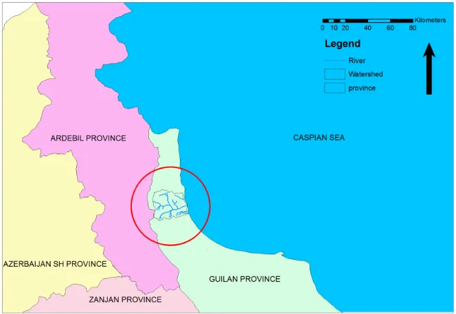
The study area is Korganrood watershed (Hashtpar City), which is located in Guilan Province, northern Iran (Fig 1). This area represents humid and temperate climatic conditions according the Domarten climate index [7].The statistical data used in this study were selected according to the Tank model’s input (Sugawara et al., 1984). Accordingly, evapotranspiration, precipitation and daily discharge data (recorded by the Ministry of Energy) were used at daily scale. The logarithmic transformation method (Log10 x+1) was applied to rescale and normalize data distribution [8]. This transformation would leads us to find the best mathematical fit between observed and expected data during simulation, but for a realistic interpretation, simulated results were de-transformed to their real scales. The Tank model assumes the watershed as a series of storage vessels and the data required for model calibration are just precipitation, evapotranspiration and observed runoff. So, we applied the Tank model as a hydrological lumped platform to simulate rainfall-runoff process at the watershed scale (Fig 2). in this regard, A summation of all the lateral water flows is equal to a calculated water discharge (QC), such as follows [9, 10]:

... (2.13)

optimization strategies (searching algorithms and objective functions) was undertaken using Pearson

coefficient of correlation (r), and eight common descriptive statistics such as mean, median, minimum, maximum, standard deviation (SD), coefficient of variation (CV), skewness and kurtosis. Pearson

1 1 1 2

1 A B C D

A

C

Y

Q

=

+

Investigating the Optimization Strategies on Performance of ... M. S. Goodarzi et al.

(3)

coefficient of correlation and also the objective functions are presented as following (equations 1 to 4) [12].

Fig 1 Geographical location of the study area

(4)

Fig 2 Tank model structure [10]

The process of the calibration demands a procedure to examine the runoff measured through a given set of parameter values and then to adjust the parameters, if required. Prior to calibration, 18 parameters were set to initial value. These parameters will be calibrated by GA, SCE and RBN Search Algorithms regarding three objective functions (MAE, RMSE and NSE) to automatically detect the best series of parameters that will produce the best fit between actual and simulated runoff [11] For finding the best configuration of the model, the Tank model will be calibrated through different collections of daily rainfall-runoff data and the learning mechanism in dependent of the type of search. Therefore, the adjusted value (for each series) at calibration step will be applied as prediction value at the verification step. Evaluation of the model performance (determining the differences between observed and predicted values) regarding

Pearson Coefficient of Correlation (r):

... (1)

Mean Absolute Error (MAE):

... (2)

Root Mean Square Error (RMSE):

(

)

÷

ø

ö

ç

è

æ

´

=

å

= = = 2 1 2 1 1 N i i N i i N i i i

Qc

Qo

Qc

Qo

r

å

=

-=

N

i i i

Qo

Qc

N

MAE

1

(5)

... (3)

NSE-Sutcliffe (NSE):

... (4)

3. Result and Discussion

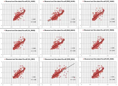
Agreement index values of the transformed data (0.708) (between rainfall and runoff records) in comparison with their original values (0.513), which would be good introduction for well rainfall-runoff modeling (hydrological series are capable to be modeled in perfect way). Calibration process was performed to achieve the best set of eighteen tank model’s parameters using the transformed data (Podger, 2005). This process consists of calibration and verification steps through which all parameters are firstly adjusted (optimized) and then assigned as prediction coefficients, respectively. Scatter plot results of simulated and observed plots are shown in Figure (3). Statement of the results was undertaken as the following steps.

A) Case Scale:

Accordingly, the best general agreement between observed and simulated runoff (regarding the coefficient of correlation) are provided as the following for calibration and verification steps, respectively (in descending format):

Calibrationstep:SCE*MAE (0.906) > SCE*NSE (0.884) > GA*MAE (0.852) > SCE*RMSE (0.825) > GA*NSE (0.799) > GA*RMSE (0.764) > RNB*RMSE (0.681) > RNB*NSE (0.608) > RNB*MAE (0.514)

Verification step: GA*RMSE (0.868) > GA*NSE (0.864) > GA*MAE (0.862) > SCE*NSE (0.852) > SCE*MAE (0.842) > SCE*RMSE (0.839) > RNB*RMSE (0.795) > RNB*NSE (0.781) > RNB*MAE (0.613).

(

)

2

1

1 å

=

-=

N i i i

Qo

Qc

N

RMSE

(

)

å

= = =

÷

ø

ö

ç

è

æ

-=

N i N i i i N i i i

Qo

N

Qo

Qc

Qo

NSE

1 2 1 1 2

1

(6)

(7)

A) Calibration (Blue) and B) Verification (Red) Fig 3 Scatter plots between observed and simulated runoff;

(8)

B) Group scale:

In order to better understand the adopted strategies, the results of optimizers and objective functions could be compared as group wise. Hence, general agreement between observed and simulated runoff at group scale was calculated. The results for calibration and verification steps are derived as the following:

SCE calibration group (average of all objective functions) is 0.871

GA calibration group (average of all objective functions) is 0.805 RNB calibration group (average of all objective functions) is 0.601 NSE calibration group (average of all search algorithms) is 0.762

MAE calibration group (average of all search algorithms) is 0.757 RMSE calibration group (average of all search algorithms) is 0.756 GA verification group (average of all objective functions) is 0.864

SCE verification group (average of all objective functions) is 0.844 RNB verification group (average of all objective functions) is 0.729 RMSE verification group (average of all search algorithms) is 0.834

NSE verification group (average of all search algorithms) is 0.832 MAE verification group (average of all search algorithms) is 0.772

4. Conclusion

As the case-wise results (part 3.2 A, and scatter plots on Figure 3.3), the best and the weakest agreement indices respectively can be seen through the combination of SCE as a searching algorithm and MAE as an objective function (SCE*MAE 0.906) and RNB as a searching algorithm and MAE as an objective function (RNB*MAE 0.514) in calibration step. Also, the best and the weakest combinations of the verification step, respectively, were retrieved from GA as a searching algorithm and RMSE as an objective function (GA*RMSE 0.861) and RNB as a searching algorithm and MAE as an objective function (RNB*MAE 0.613). According to the group-wise results (part 3.2 B), the best and the weakest agreements are respectively related to the SCE calibration group (0.871) and RNB calibration group (0.601). The results for objective functions are NSE calibration group (0.763) and RMSE calibration group (0.756). In addition, the best and the weakest agreement results for verification groups are depicted respectively for GA (0.864) and RNB (0.729). The results for objective functions are RMSE calibration group (0.834) and MAE calibration group (0.772).

The cross investigation of the top optimization strategies with descriptive statistics indicated that SCE*MAE has a great ability on kurtosis (-3%), skewness (-6%), median (+7%) and mean (+1%) modelling; moderate ability on maximum (-23%), standard deviation (-33%) and coefficient of variation (-34%) modelling; and inability on minimum (+1300%) modelling. GA*RMSE also has a great performance on median (+2%); moderate ability on mean (-11%), standard deviation (-39%), coefficient of variation (-32%), skewness (-28%); and inability on minimum (+50%), maximum (-56%) and kurtosis (-71%) modelling (irrespective of their total r2_{agreement with observed values). A}

remarkable finding of this study is directly related to the dependency of the results in terms of ecological and climatological attributes of the study area. Therefore, conducting a complementary study using a wide range of watersheds and considering different attributes (as a hydrological unit) is critically suggested to promote the generalizability of the findings. Finally; according to the importance and necessity of each parameter’s role in modelling the process and also for better understanding of the model’s outputs, in future related researches, a sensitivity analysis method is suggested to apply for the total set of 18 parameters of the Tank hydrological model.

(9)

References

[1] Bonacci, O. (2004). The Basis of Civilization: on the role of hydrology in water management - Water Science? (Proceedings of the UNESCO/IAHS/IWHA symposium held in Rome, December 2003) . IAHS Publ. 286.

[2] Wagener, T., & Gupta, H. V. (2005). Model identification for hydrological forecasting under uncertainty, Stochastic Environ. Res. Risk Assess., 19, 378–387,doi:10.1007/s00477-005-0006-5. [3] Sugawara, M., Watanabe, I., Ozaki, E., & Katsuyama, Y. (1984). Tank Model with Snow Component. Research note no, 65. National Research Center for Disaster Preventation, Japan. 293p. [4] Goldberg, D. E. (1989) Genetic Algorithms in Search, Optimization, and Machine Learning. Addison Wesley, Boston, USA.

[5] Rosenbrock, H. H. (1960). An automatic method for finding the greatest or least value of a function. Comput. J. 7, 175–184.

[6] Divya, B., & Ashu, D. (2010). Comparison of Various Search Algorithms for Calibration of Conceptual Rainfall-Runoff Models. EGU General Assembly 2010, held 2-7 May, 2010 in Vienna, Austria, p.9463.

[7] Sheikh Goodarzi, M., Sakieh, Y., Navardi, S. (2016). Scenario-based urban growth allocation in a rapidly developing area: a modeling approach for sustainability analysis of an urban-coastal coupled system. Environ Dev Sustain (2016). doi:10.1007/s10668-016-9784-9. Pp:1-24

[8] LEADTOOLS. (2006). SPSS for Windowse. Ver 15.0. Copy right© LEAD Technologies Inc. [9] Setiawan, B. I., yanto, R., Ilstedt, U., & Malmer, A. (2007). Optimization of Hydrologic Tank Model’s Parameters. Swedish University of Agricultural Sciences, Department of Forest Ecology, Umeå, Sweden.

Garrick, M. , Cunnane, C., & NSE, J. E. (1978) A criterion of efficiency for rainfall-runoff model. Hydrol. 36, 375-381.

Lauzon, N., Rousselle, J., Birikundavyi, S., & Trung, H.T. (2000). “Real-time Daily Flow Forecasting Using Black-box Models, Diffusion Processes and Neural Networks”, Can. J. Civ. Eng. 27, 2000, pp 671-682.

[10] Podger, G. 2005. Rainfall Runoff Library (RRL). Catchment Modeling Toolkit prepared by the © CRC for Catchment Hydrology, Australia. Pp: 110.

[11] Nash, J. E., & Sutcliffe, J. V. (1970) River flow forecasting through conceptual models, Part 1, A discussion of principles. J. Hydrol. 10, 282–290.

[12] Lauzon, N., Rousselle, J., Birikundavyi, S., & Trung, H.T. (2000). “Real-time Daily Flow Forecasting Using Black-box Models, Diffusion Processes and Neural Networks”, Can. J. Civ. Eng. 27, 2000, pp 671-682.