Analysis of the Kernel Bandwidth Influence in the Double Smoothing Merging Algorithm to Improve Rainfall Fields in Poorly Gauged Basins

Analysis of the kernel bandwidth influence in

the double smoothing merging algorithm to

improve rainfall fields in poorly gauged basins

Nicolás Duque-Gardeazábal

_{, David Zamora}

_{and Erasmo Rodríguez}

[email protected]

Abstract

Accurate estimates of precipitation are needed for many applications in hydrology as rainfall is one of the most influential variables of the water cycle. The common sources of information used to estimate rainfall fields are in situ rain gauges, remote sensing information and outputs from climate models. However, each of the above-mentioned sources has its own limitations, which can be reduced by blending information from these sources, in a product that takes advantage of the strengths of each dataset. In this research we study the double smoothing merging algorithm, creating a rainfall distributed product that combines remote sensed and reanalysis data, and information from a rain gauge network. The main objective of the study is to investigate the implications of varying the rain gauge density and configuration, on the merging parameters and global performance of the blended product. The results of a daily 3-year period experiment show that, although the errors in cross validation (CV) and against an independent dataset (IV) are in general low, the performance of the blended product and also the sensitivity of the parameters are highly influenced by the rain gauge configuration and density. The bandwidth merging parameters increase as the network density is artificially reduced.

1

Introduction

From the variables of the water cycle, rainfall is one of the most influential because surface and subsurface water availability depend on it. Rainfall is recognized as one of the main forcings of the terrestrial water cycle (Chow, Maidment, & Mays, 1988). Accurate estimates of precipitation are needed for many applications in hydrology, meteorology, agriculture, risk assessment, etc (García,

* _{Made the calculations and wrote most of the text} † _{Gave advice regarding the text and the methodology} ‡ _{Gave advice regarding the text and the methodology}

Volume 3, 2018, Pages 635–642

Rodríguez, Wijnen, & Pakulski, 2016). A typical use of distributed rainfall estimates is as forcing for hydrological and land surface models (Silberstein, 2006), as well as input for water indices calculation.

There are many procedures used to estimate rainfall fields. The most common approach is to derive them from point observed data using interpolation methods, such as the geostatistical and traditional methods mentioned by Grimes & Pardo-Iguzquiza (2010), yet they are highly dependent on the network density and spatial configuration. Besides, around the world rain gauge networks are being reduced (e.g. see (García et al., 2016)). In Colombia and also in its Orinoquia and Amazonian territories (which are characterized by a low measurement density), estimating rainfall fields based only on in situ data is challenging.

Other sources of rainfall information come from either remote sensing or climate models. The simulation of precipitation that the latter do, exhibit biases due to the complex and coupled processes of water and energy fluxes. Although remote sensing products have become more relevant in water resources projects, they also have uncorrected biases and therefore, are in general not suitable for hydrological applications that require for example daily rainfall data (Serrat-Capdevila, Valdes, & Stakhiv, 2014). However, merging remote sensing or climate simulated products with rain gauge estimates has significant advantages (Li & Shao, 2010). Several methodologies to blend remote sensed data and point estimates have been proposed in the literature, e.g. conditional merging, bias correction, geostatistical estimation methods, among others (Jongjin, Jongmin, Dongryeol, & Minha, 2016). A particular statistical approach which is not based on Gaussian and stationary assumptions, and that is emphasised for data sparse regions, is the so-called double-kernel smoothing (DS), proposed by Li & Shao (2010). This merging algorithm is flexible since it only requires the rain gauge and remote sensed data coordinates, and their time series, allowing to easily introduce or retrieve additional rain gauges or changing the remote sensed product, without having to implement other pre-processing algorithms, such as variogram calculation and fitting.

The focus of this study is to evaluate, in a tropical complex high relief terrain, the performance at daily timescale of the DS method constrained by the density of rain gauges. In order to do this, we focus on both, calibrating merging kernel parameters (h1 and h2) and evaluating their variation with gauge density. In addition, to the in situ data, we used the 0.25° gridded Multi-Source Weighted-Ensemble Precipitation (MSWEP) (Beck et al., 2016).

2

Materials and Methods

The study area corresponds to the Sogamoso River basin in Colombia, a watershed densely instrumented, located in the Andean Mountains, with an area of 20,300 km2. Within this watershed there are 219 rain gauges, and from those, 156 stations with more than 50% of daily rainfall observations available for the period 1980-2012 were selected for analysis. Average annual precipitation in this watershed is approximately 1,600 mm, varying between 800 mm to 3,000 mm. We studied the blending of the in situ daily rainfall information with the MSWEP, retrieving the rain gauges that were used to create the global product.

The rainmerging R package (Zulkafli, Nerini, & Manz, 2015) was used to perform the blending between the MSWEP and the in situ rain gauge information. First, we performed a merging with fixed parameters using the Silverman’s rule of thumb (Silverman, 1986) in order to analyse the spatial effects of merging the MSWEP with the rain gauge network. In the merging algorithm, the first parameter is the bandwidth associated with the “weighting of the surrounding observations by distance” Li & Shao (2010), while the second parameter is related to the weighting based on the distance of the pseudo-observations. The Silverman’s rule varies the h1 value when rain gauges are artificially retrieved, whereas the h2 value does not vary since the pseudo observations are estimated in the same coordinates where predictions are made. Averaged Silverman’s values are showed in Table 2. We then modified the DS.R algorithm to allow the calibration of the kernel bandwidth parameters (h1 and h2).

Category 100% 70% 50% 30% 10%

h1 (km) 4.75 5.16 5.44 6.00 8.16

h2 (km) 3.42 3.42 3.42 3.42 3.42

Table 2: Averaged parameters values calculated with the Silverman’s rule

An experiment was conducted during the 1994-1996 period at daily time scale, in which the different richness levels of information were used to explore the merging technique features. The reason behind choosing these years was that one positive and one negative phase of the ENSO climatic phenomenon occurred in the 3-year period. This experiment gave some insights about the behaviour of the calibrated merging parameters both in CV and IV; the performance of the blended products for the different network configurations was based on the RMSE. Due to the extensive time that the CV mode consumes and the complex objective function surface that was expected, the Shuffled Complex Evolution algorithm (SCE-UA) (Duan, Sorooshian, & Gupta, 1992), was chosen to calibrate the merging parameters. We also used the GLUE algorithm (Beven & Binley, 1992) to sample the parameter space and we also performed a sensitivity analysis of the parameters, but only in the IV mode. The sensitivity analysis was performed using the Monte-Carlo Analysis Toolbox (MCAT) (Wagener, Lees, & Wheater, 2001), which ranks the uniform random sampled parameters with respect to their objective function into 10 groups of equal size, as proposed by (Freer, Beven, & Ambroise, 1996). This has the aim of avoiding the subjectively chosen threshold value that divides the so-called behavioural and non-behavioural simulations stated by (Beven & Binley, 1992).

Additionally, the “raw” MSWEP data was evaluated against the rain gauges. This comparison was first made against the rain gauges that comprise each category and each configuration, allowing to obtain the RMSE for the same gauges used in the CV mode. Then, the evaluation was performed against the independent gauges considered in each category and configuration. As a result of this analysis we calculate RMSE with the same gauges used in the IV procedure but just assessing the MSWEP performance.

Through line plots, the values of RMSE and the kernel bandwidths for each density category and each network configuration were analysed for both CV and IV modes.

Category 100% 70% 50% 30% 10%

Number of rain gauges in analysis and CV 156 109 78 46 15 Rain gauge density (gauges/1000 km2) 7.69 5.38 3.85 2.27 0.74 (km2/gauge) 130 186 260 441 1354 Number of Realisations (Configurations) (Conf) 1 3 3 3 3 Number of rain gauges in Ind. Validation (IV) Not apply 47 78 110 141

3

Results and discussion

Figure 1 shows, for a selected date (January 1st , 1980), the original MSWEP estimated field and the merging results between this product and two rain gauge networks with different densities; gauges are depicted as points in Figures 1a, b and c; rain amount is associated with the blue scale colour. It can be observed in Figure 1 that although the merging procedure is mainly driven by the rain gauge values, it still captures some of the patterns registered on the MSWEP product. It also can be seen in Figure 1 that there are isolated gauges that produce some precipitation bull’s eyes. The influence of the bandwidth is clear around these isolated gauges, where the rainfall amount smoothly diminishes close to the gauge and in this case influences the first line of cells around the rain gauges. Figure 1c shows that even with a low gauge density (30%), the DS method still captures the main spatial pattern showed in Figure 1b for the 100% category, where the rain registered at the north of the basin was estimated by the MSWEP (Figure 1c), and those values were adjusted by the procedure based on the few gauges that are located on that zone. Although there are a few specific locations in Figure 1b where a considerable amount of rain was registered (e.g. at the cells on the West of the basin), the blending using the gauges considered in the 30% category was not able to reproduce them. The latter remarks the influence that a rain gauge network configuration have in the final estimated rainfall field.

Figure 1: a) Rainfall field derived from the MSWEP, and rainfall fields estimated with the DS using Silverman’s rule with b) 100% and c) 30% of rain gauges. Missing values for 01/01/1980 are red points

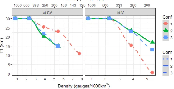
The parameter and error results of the 3-year calibration experiment are depicted in Figure 2, 3 and 4. The RMSE and the optimized values of the kernel bandwidths are highly dependent on the network configuration. Figure 2 shows the h1 kernel bandwidth results for the CV and IV, Figure 3 depicts the results for h2, while Figure 4 displays the RMSE. In both validation strategies, in general, the calibrated h1 kernel bandwidth tends to increase as the gauge density declines, result that is expected, as this is the parameter that is related to the distance between the gauges and the center of the grids. In the IV evaluation (see Figure 2b), the increasing trend in h1 appears to be equally stable as in CV mode, as the 3 configurations analysed performed in a similar way.

The h2 kernel bandwidth considerably varies across the different densities and configurations analysed. It reports a tendency to increase with the artificial decline in network density, and largely changes with configuration, meaning that this parameter is more influenced by the rain gauge configuration than by the rain gauge density (Figure 3). The differences between Figures 3a and 3b maybe also due to the number of gauges that are used to calculate the performance; IV compares the estimates with more gauges than each pseudo-field iteration created in the CV.

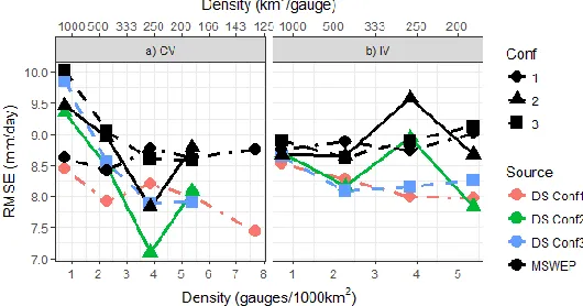
With respect to the RMSE, in both calibration strategies (CV and IV) (Figure 4), the error changes from one network configuration to the other. Yet, the errors tend to increase with the artificially reduction of the rain gauge density. Furthermore, the RMSE appears to stabilize after the 3

Figure 4: RMSE in the 3-year calibration experiment evaluated through a) cross-validation (CV) and b) Independent Validation (IV) against rain gauge density. Black lines correspond to the

evaluation of the “raw” MSWEP data against each category and configuration.

gauges/1000 km2_{, probably because the merging method offsets the errors that are generated by}

reducing the gauge density. The performance of the “raw” MSWEP is highly improved when several rain gauges are considered in the blending, behaviour that is also expected. Even with a sparse network configuration, i.e. 2 or 1 gauge/1000 km2_{, the methodology still generates a slight}

improvement over the performance of the “raw” MSWEP and probably a bigger enhancement if it was compared against a rain gauge interpolation from a reduced number of point observations.

Because of the different number of gauges used to accomplish the evaluation of the two validation strategies, a particular behaviour can be identified for Conf 2, at the category 3.85 gauges/1000 km2. Figure 4a shows that in the CV mode the influence of the rain gauge configuration is strong, since the 3.85 gauges/1000 km2 density has anomalous low error for Conf 2 whereas the other two configurations performed slightly similar. Although in CV mode this configuration reports a low error, in IV mode it has the highest error (Figure 4b). A reason that could explain this is that there is an important number of rain gauges, or a group of them, that is not considered in the merging procedure, but they are included in the IV gauges. Hence, the IV methodology reports a large error; while in the CV mode it creates a false good performance result.

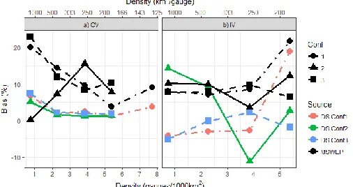
An analysis of the Percent Bias, using both evaluation strategies, is plotted in Figure 5. It is clear from Figure 5a, which shows the results in the CV mode, that the merging between the MSWEP and the rain gauges reduces the bias of the estimated field. The reduction varies from 5% to 20% depending on the gauge density that has been used, also all the configurations reports a similar behaviour. Even though the performance in poor densities decreases to a positive bias (feature that stems from the MSWEP), there is a considerable reduction of the Bias. The results using IV gauges are displayed in Figure 5b. The MSWEP also reports an approximate 10 % positive Bias in nearly all configurations while the DS merging results are mix between positive and negative Bias. Yet, two out of the three configurations are near 0 % for the less dense rain gauge configurations. These results evidence the ability of the procedure, not only to reduce the overall error, but also to reduce the Bias of the distributed field.

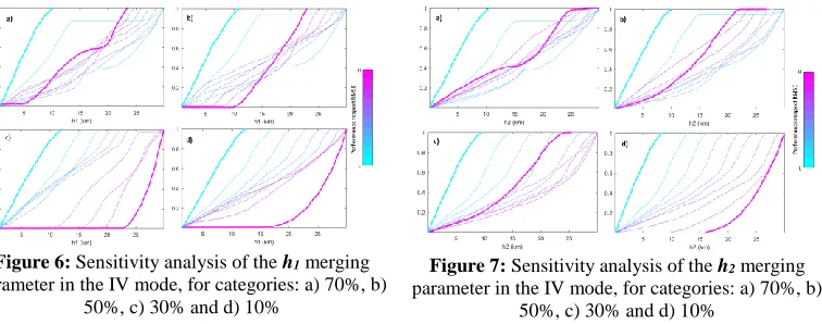
Regarding the sensitivity analysis, both parameters are identified as sensible. Figure 6 depicts the regional sensitivity plots for the h1 merging parameter for the categories 70, 50, 30 and 10 %. It can be seen that regardless of the rain gauge density, the sensitivity of the parameter increases with the artificially reduction of gauge density, since the 30% and the 10% categories have large differences between the lowest and the highest performance frequency distributions. Moreover, the best distributions move towards higher values when the rain gauge is artificially reduced, e.g. for the 70% of original gauges the most probable value is around 15 km, whereas at 30% the most probable is

Figure 5: Percent Bias in the 3-year calibration experiment evaluated through a) cross-validation (CV) and b) Independent Validation (IV) against rain gauge density. Black lines correspond to the

around 25 km. The estimated value given by Silverman’s rule are far below the calibrated values (see Table 2), fact that highlights the importance of parameter calibration. This analysis complements the results related to the variation of the optimized parameter shown in Figure 3.

Figure 7 portrays the sensitivity plots for the h2 merging parameter. Although the graphs show that the parameter is sensible, regardless of the configuration, it is not as sensible as the h1 parameter since the cumulative distributions are not so disperse, compared with those depicted in Figure 6. This result is very different from the values estimated by the Silverman’s rule (3.42 km for the h2 merging parameter) and they remark the importance of calibrating the parameter. Furthermore, it can be seen that the cumulative frequencies have an approximate constant rate, meaning that it is not completely probable to find the optimum value for this parameter in a certain interval (10 % category is an exception that can stem from the low rain gauge density).

4

Conclusions

The DS satellite-raingauge merging procedure, developed for poorly instrumented basins, has been implemented and tested in a basin in Colombia, using a 3-year calibration experiment conducted over 5 different rain gauge density categories and 3 different network configurations for each category.

The results showed that there is a trend on the first merging parameter (h1) to increase its calibrated value with the reduction of the rain gauge network density. The second merging parameter (h2) does not appear to have a clear correlation with the gauge density. The RMSE seems to stabilize after a density of 3 gauges/1000 km2, possibly because the satellite precipitation maintains consistent estimates where rain gauge density is low. Also, the overall Bias is reduced. This is a good sign of the ability of the method to create reliable rainfall fields in data scarce regions, e.g. in watersheds with a network density lower than 3 gauges/1000 km2, because the error does not increase significantly when the rain gauge network density is reduced to less than 1 gauge/1000 km2. Moreover, the results highlight the possibility to increase the performance of distributed rainfall field with a flexible procedure, which allows to easily introduce or retrieve certain gauges or change the remote sensed estimates.

However, it is clear that the results are highly affected by the network configuration. The RMSE and the value of the parameters varied significantly from one realisation to the other, yet the procedure reduces the Bias of the remote sensed product. The validation against the independent set of rain gauges seems to be more reliable than the cross-validation, since the rainfall field is being compared to more gauges than in the cross-validation and is also faster, as just one estimate must be

Figure 6: Sensitivity analysis of the h1 merging parameter in the IV mode, for categories: a) 70%, b)

50%, c) 30% and d) 10%

Figure 7: Sensitivity analysis of the h2 merging parameter in the IV mode, for categories: a) 70%, b)

done. This statement appears to be corroborated by the stable trends in the h1 merging parameter. Nevertheless, the independent validation is just appropriate to implement in rich data regions where the influence of a few gauges, not considered in the blending, would be low. Additionally, the cross-validation is computationally demanding and for the calibration of the parameters, metaheuristic calibration procedures may also be used.

The sensitivity analysis allows to conclude that both merging parameters must be calibrated. It also confirms that the possible optimum values of the h1 parameter increase when there is a poor gauge measurement density, whereas the optimum value of the h2 parameter appears to not have a most probable value (10 % category is an exception that can stem from the low rain gauge density).

The blending techniques must also be evaluated against the classical interpolation procedures, such as Inverse Distance Weighting (IDW), Kriging and its derivates (Residual Kriging, Universal, with External Drift, etc.). This would allow to evaluate how much the merging of products can improve rainfall estimates and therefore water resources accounting and management in data sparse regions. An interpolation using the procedures mentioned above is under progress and methods are being applied in the same categories and configurations used for the blending.

References

Beck, H. E., van Dijk, A. I. J. M., Levizzani, V., Schellekens, J., Miralles, D. G., Martens, B., & de Roo, A. (2016). MSWEP: 3-hourly 0.25° global gridded precipitation (1979-2015) by merging gauge, satellite, and reanalysis data. Hydrology and Earth System Sciences Discussions, 0(May), 1-38. https://doi.org/10.5194/hess-2016-236

Beven, K., & Binley, A. (1992). The future of distributed models: model calibration and uncertainty prediction. Hydrological Processes, 6(May 1991), 279-298. https://doi.org/10.1002/hyp.3360060305

Chow, V. Te, Maidment, D., & Mays, L. (1988). Applied Hydrology. Singapore: McGraw-Hill Book Co. Duan, Q., Sorooshian, S., & Gupta, H. V. (1992). Effective and efficient global optimization for conceptual rainfall-runoff models. Water Resources Research, 28(4), 1015-1031. https://doi.org/10.1029/91WR02985

Freer, J., Beven, K., & Ambroise, B. (1996). Bayesian estimation of uncertainty in runoff prediction and the value of data: An application of the GLUE approach. Water Resources Research, 32(7), 2161-2173. https://doi.org/10.1029/96WR03723

García, L. E., Rodríguez, D. J., Wijnen, M., & Pakulski, I. (2016). Earth Observations for Water Resources Management: current use and futute opportunities for the water sector. Washington D.C.: International bank for recostruction and development/ The world Bank.

Grimes, D. I. F., & Pardo-Iguzquiza, E. (2010). Geostatistical Analysis of Rainfall. Geographical analysis, 42, 136-160. https://doi.org/10.1111/j.1538-4632.2010.00787.x

Jongjin, B., Jongmin, P., Dongryeol, R., & Minha, C. (2016). Geospatial blending to improve spatial mapping of precipitation with high spatial resolution by merging satellite-based and ground-based data. Hydrological Processes, 2803(March), 2789-2803. https://doi.org/10.1002/hyp.10786

Li, M., & Shao, Q. (2010). An improved statistical approach to merge satellite rainfall estimates and raingauge data. Journal of Hydrology, 385(1-4), 51-64. https://doi.org/10.1016/j.jhydrol.2010.01.023

Serrat-Capdevila, A., Valdes, J. B., & Stakhiv, E. Z. (2014). Water management applications for satellite precipitation products: Synthesis and recommendations. Journal of the American Water Resources Association, 50(2), 509-525. https://doi.org/10.1111/jawr.12140

Silberstein, R. P. (2006). Hydrological models are so good, do we still need data? Environmental Modelling and Software, 21(9), 1340-1352. https://doi.org/10.1016/j.envsoft.2005.04.019

Silverman, B. W. (1986). Density Estimation for Statistics and Data Analysis. (Chapman & Hall/CRC, Ed.). London.

Wagener, T., Lees, M., & Wheater, H. (2001). Monte-Carlo Analysis Toolbox. London. Recuperado a partir de http://www.imperial.ac.uk/environmental-and-water-resource-engineering/research/software/