Vol. 8, No. 2, 2014, 27-36
ISSN: 2279-087X (P), 2279-0888(online) Published on 17 December 2014
www.researchmathsci.org
27
Annals of
A Study on Numerical Stability of Finite Difference
Formulae for Numerical Differentiation and Integration
M. Ramesh Kumar1 and G. Uthra2
1
Department of Mathematics, Saveetha Engineering College, Thandalam Chennai-602105. India. Email: [email protected]
2 PG & Research Department of Mathematics, Pachaiyappa's College
Chennai- 600030, India. Email: [email protected]
Received 3 September 2014; accepted 21 November 2014
Abstract. The numerical differentiation based on the interpolating polynomial is basically
an unstable process and one cannot expect good accuracy even when the original data are known to be accurate. We analyze the stability of computation of derivatives through polynomial interpolation at given point numerically and prove it has poor stability when closer to the interpolating nodes however it has a quite good stability between interpolating nodes.
The numerical integration by use of lower order formulas such as trapezoidal rule and Simpson rule gives accuracy of results than use of higher order Newton-Cotes formulae. In this paper, we also analyze the reason for the poor stability of higher order Newton-Cotes formulae. Numerical examples are given to study roundfoff error analysis of numerical differentiation and integration.
Keywords: Round off errors, numerical differentiation, integration, Newton-Cotes
formulae, numerical stability
AMS Mathematics Subject Classification (2010): 65D25, 65D30
1. Introduction
Numerical approximations to derivatives are used mainly in two ways. First, we are interested in calculating derivatives of given data that are often obtained empirically. Second, numerical differentiation formulae are used in deriving numerical methods for solving ordinary and partial differential equations. The problem of numerical differentiation of noisy data is ill-posed, small changes of the data may result in large changes of the derivative. There is always a conflicting relationship, as nodes become denser, data reflect the rapid variation better while differentiation of the data gets more noise. Consider the central difference formula for approximating
(1)
28
′ ∆ ∆ ′′′
Hence
′ ′
∆∆
′′′
(2)
The error in the computed approximation of ′
and ′ is therefore seem to consist of two parts, one part due to roundoff, and the other part due to discretization. If
′′′
is bounded, then the discretization error goes to zero as 0, but the round off error goes if we assume that ∆ ∆ does not decrease. Hence, ′ gives good approximation only at optimum value of . If is small and approaches to zero i.e when the data is dense then the process estimating derivatives for evenly spaced nodes is unsatable. This analysis shows that we can combat the round off error by using “sufficiently” high precision arithmetic. But this is impossible when is only approximately at finitely many points [1]. However, in Ref[5] shows that the use of a higher-order formula, such as a 7-or even a 10-point approximation, based on the method of undetermined coefficients, can sometimes lead to better accuracy and enhanced computational efficiency rather than 2- point and three point formula. In the present study we give roundoff error analysis for higher order numerical differentiation formula through polynomials for arbitrary spaced grids. In this paper, we give the round of errors of calculation of derivatives through polynomial interpolation and analyze the stability of numerical differentiation up to higher order.
The idea of numerical integration is to replace a complicated function or tabulated data with an approximating function that is easy to integrate. Polynomial function is the best choice to replace the actual function because of its simple form and also it can be easily found through Lagrange interpolation formula or Newton interpolation formula[4] for evenly or unevenly spaced grids with any degree of accuracy. If the nodes are spaced evenly then the quadrature formula is called Newton-Cotes formula. Trapezoid, Simpson’s 1/3 and 3/8 rules, Bode’s are special cases of 1st, 2nd, 3rd and 4th order polynomials are used, respectively in Newton cotes formulas. Using large number of equally spaced nodes may be inaccurate behavior associated with high-degree polynomial interpolation Indeed, every n-point Newton-Cotes rule with n ≥ 11 has at least one negative weight, so Newton-Cotes rules become arbitrarily ill-conditioned. The lower order formulas for approximating integrals such as Trepezoidal and Simson rules are special cases of Newton-Cotes integration formulas and gives better accuracy then higher order formulas. In this paper we analyse poor stability of higher order Newton-Cotes formula through roundoff error analysis.
2. Preliminaries
Let !" denote the vector space of all polynomials of degree at most # and let $, &
0, . . . , #, be # 1 distinct nodes and suppose that $, & 0, . . . , #,, are corresponding numbers. Then, there exists a unique polynomial )* Π+ such that ) $, &
Differentiation and Integration
29
12 ∏ "45. 4 and 1$,2 ∏ 6667
867
" 45.,
$94 . (3)
The Lagrange’s interpolation formula[1, 3] for approximating on the X is given by
),2 ∑ 1"$5. 2,$$. (4)
Differentiating ; times with respect to ,
),2< ∑ 1"$5. $,2<$, (5)
where ),2< and 1$,2< are ;= derivatives of ),2 and 12,$ respectively. Let > -?., ?, ?, … , ?"0 and denote the Lagrangian polynomials as follows
1@A ∏ A ?"45. 4 and 1$,@ ∏ CBC7
8C7
" 45.,
$94 . (6)
The Lagrange’s interpolation for approximating on ser J is given by
),@A ∑ 1"$5. $,@$. (7)
Definition 2.1. Define the condition number of ;= order derivative of ),2 at x for
# D EF-00 over the set X as follows[3]
cond,, , supNDOlim .STU,V
W6T
UX∆U,VW 6S
STU,VW6S (8)
Similarly, condition number of ;= order derivative of ),@ at s over the set J as follows
cond>, A, supBD@lim .STU,Y
WBT
UX∆U,YW BS
STU,YWBS (9)
3. Round of error analysis of numerical differentiation
Define minZ-|$ |0 \ 0 for & 0, . . . , # and arrange each node $, &
0, . . . , # by spacing at distance ?$ from ., (i.e) $ . ?$, where ?. 0, ?"
" ./ and satisfies 0 ^ ?$ ^ " ./. Let be any point on _., "` and
. A, where 0 ^ A ^ " ./. Then, the following relationship holds between Lagrange’s polynomials (3)
30 Using (3), (6) and (8) gives
),2 ∑ 1"$5. $,2$ ∑ 1"$5. $,@A$
Thus, we find that
),2 ),@A (12)
Equation (12) shows that ),2 does not depend on . Differentiating (11) with respect to and using aA a/, gives
b6b c1$,2d b6b c1$,@Ad
bBb c1$,@Ad ebBb6
bBb c1$,@Ad
bBb c1$,@Ad ebBbB
1$,2 1$,@A
Differentiating again with respect to , gives
1$,2 1$,@A
Proceeding this ; times, yields
1$,2< W1$,@<A (13)
Substituting (13) in (5), gives
),2< W∑ 1"$5 $,@<A$
′ .
(14)
Let ∆ is the small change in . Then
)∆,2< W∑ 1"$5. $,@<A$ ∆$ (15) (14)-(5) f
Differentiation and Integration
31
S),2< )∆,2< S ^W∑ S1"$5. $,@<A∆$S
Choose |∆| g *, gives
S),2< )∆,2< S ^hW∑ S1"$5. $,@<A$S (16)
Equality is attained for ∆$ sign*$ 1$,@<?$
S),2< )∆,2< S W∑ 1"$5. $,@<A$ (17)
Similarly, we easily find that
S),@<A )∆,@< AS ∑ 1"$5. $,@<A$ (18)
Using (17) and (18) , gives
STU,Y
WBT
UX∆U,YW BS
STU,YWBS
STU,VW6TUX∆U,VW 6S
STU,VW6S
Hence,
cond,, , cond>, A, (19)
Hence the condition number on X at x is same as condition number J at s
Using (16) and (19), yields the bound for roundoff error of ),2<
S),2< )∆,2< S ^hW cond>, A, S),@<AS (20)
Suppose that be a real-valued function and continuously differentiable function on the closed interval _, j`, klml min-., . . . "0 and
j max-., . . . "0 . Shadrin [8] has shown that if ),2 denotes the polynomial of degree n interpolating f at the points ., , … " then for ; 0, 1, … , #
S),2< <S ^ p12<p p<!WXp. (21)
This bound was earlier conjectured by Howell [3] who also proved it for the highest derivative r #. Let )s,2< is computed ),2<. Then
32
S)s,2< <S ^hW cond>, A, S),@<AS p12<p p<!WXp.
Using (13), we find the bound for total error
S)s,2< <S ^ *
< cond>, A, S),@<AS
"<p1@<Ap p<!WXp. (23)
3.1. Numerical experiment
We report an experiment whose purpose is to verify the conclusions of the roundoff error analysis. There are plenty of numerical differentiation formulas in literature. Here, we use following formula from [6] to compute ;= order derivative on various distribution.
W<!6t
u∑ $k$,2∑
7
686WX7 v<
<w 45. "
$5. x. (24)
Where . 1, ∑45.< 4y<4 0, v z1, 0, \ $
${ , y| ∑
686}X
"
$5. and x
12 ∑<w45. "4<!~X7XW7 . The computations were performed in MATLAB, for which
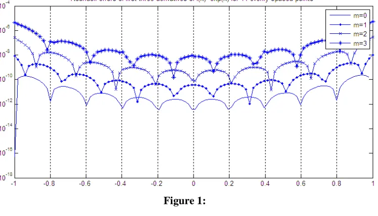
10. In first example, we take 11 equally spaced points C on _1,1` thus # 10 and set eN. We evaluate the derivatives approximately up to order 3 at 100 equally spaced points. Figure 1 and Figure 2 plots the errors for derivatives up to order 3 for 11 points on evenly spaced points and Chebyshev points of first kind.
Differentiation and Integration
33 Figure 2:
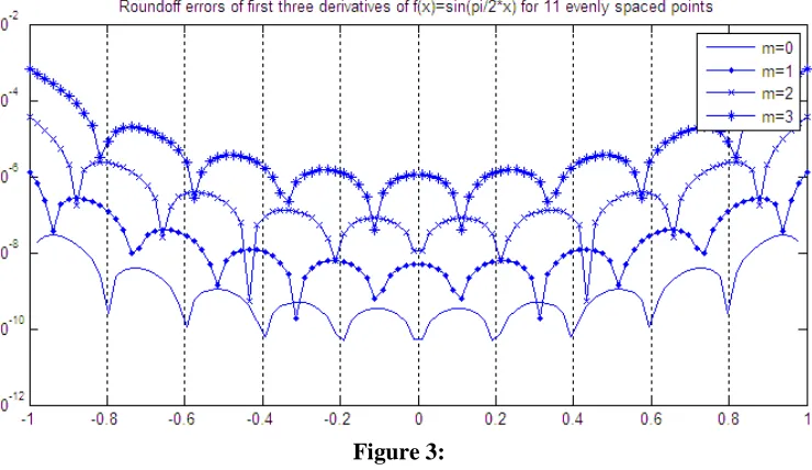
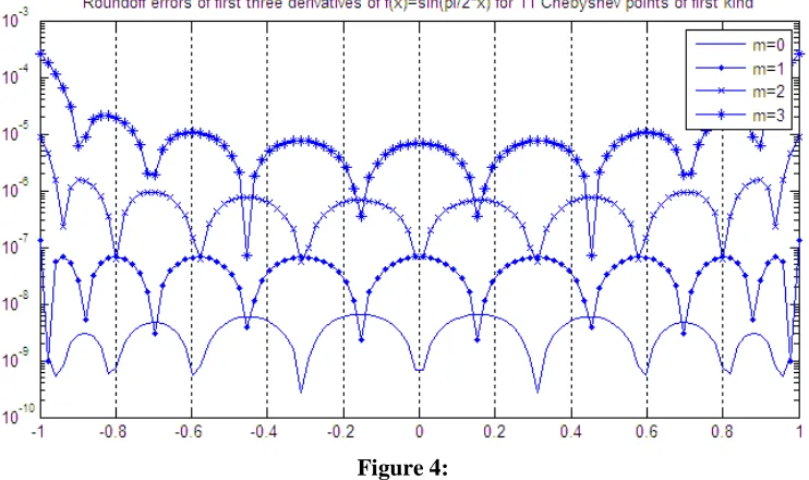
In the second example, we take 11 equally spaced points C on _1,1` thus # 10 and
set sin π. We evaluate the derivatives approximately up to order 3 at 100 equally spaced points. Figure 3 and Figure 4 plots the errors for derivatives up to order 3 for 11 points on evenly spaced points and Chebyshev points of first kind.
34 Figure 4:
The equation (23) clears that computation of derivatives through finite difference formula depends upon condition number of order of derivatives and h. These are the two factors determines stability of the computation of the numerical derivatives. Usually, if the order of derivative increases then the power of h decreses in (20). This proves that the round off error increases when the order differentiation also increases. In the first example the condition number of first three derivatives of l6 on evenly spaced points are 2982.4, 79925, 1.2861 e 10. Hence the roundoff errors of higher order derivatives increases when condition number increases. In the second example the condition number of first three derivatives on evenly spaced nodes are 3.8144e 10, 4955.4, 2.816e 10. But power of h decreases when the order of differentiation increases. If h is too small the roundoff error becomes very high. Hence, the calculation of derivatives near the nodes gives very poor accuracy. For larger values of h, the discretization error in (23) becomes high. Therefore, for very few points between the nodes gives quite good accuracy.
4. Roundoff error analysis of numerical integration
Let ., , … , " are distinct numbers on the closed interval _, ` and D
"_, `. The problem of numerical integration is to approximate the definite
integral 66a. Since polynomials are easy to integrate by using Taylor series, we find that
66),2a ∑"45.4!7 ),24. (25)
Let ∆ is the small change in . Then
66),2a 66)∆,2a ∑"45.4!7 c),24 )∆,24d.
Differentiation and Integration
35
S66),2a 66)∆,2aS ^ ∑"45.4!7 ),24 )∆,24
∑"45.44! ),@4A )∆,@4A. Using (20), yields that
S66),2a 66)∆,2aS ^ * ∑ 4cond,, , TU,Y
7B
4! "
45. (26)
Newton-Cotes formulae. Let $ &,& 0,1,23, … , #, \ 0 are equally spaced grids. Now replacing by and by # in and after simplification, we obtain
S "),2a ")∆,2aS ^ * ∑ #4cond,, , TU,Y
7C
4! "
45. (27)
The equation gives roundoff error of # 1 point formula for Newton-Cotes closed integration formula. Since the open quadrature formula do not require functional value at
the limit points of integration, assume that $ &,& 1,2, … , #-1, \ 0. Then
S "),2a ")∆,2aS ^ * ∑ #4cond,, , TU,Y
7C
4! "
45. (28)
Linear multistep methods. Let ", ", ",… , " are 1 distinct numbers on the interval _", "`, where " " ′. If we approximate the differential equation ′ , by integrating from
" to ", gives S66~′),2a
~ )∆,2a
6~′
6~ S ^ *′∑
′
4
cond,, , TU,Y
7C
4! "
45.
The equation gives roundoff error of 1 point predictor formula. If we
approximate the differential equation ′ , by integrating from " to ", gives
S66~ ),2a
~′ )∆,2a
6~
6~′ S ^ *′∑
′
4
cond,, , TU,Y
7C
4! "
45.
This kind of multistep formula is known as 1 point corrector formula.
4.1. Numerical example
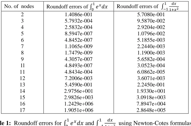
We give numerical example for roundoff errors of evaluation of integrals l. 6a and
6b6 using n-point Newton-Cotes formula. The roundoff errors of number of noes # 2,3, … ,17 are given in table 1. Trepzoidal, Simpson’s 1/3 and Simson’s 3/8 rule are special cases of Newton-Cotes formulas for # 2,3 and 4. The table 1 shows numerical instability of higher order Newton-Cotes formulas for computation of l. 6a and
6b6 .
36
Table 1: Roundoff errors for l. 6a and 6b6 using Newton-Cotes formulas for n=2,3,…,17
5. Conclusion
In conclusion, we note that roundoff error analysis numerical differentiation and integration through polynomial interpolation have been studied in this article. It is shown that the round off errors are depend on condition number of the derivative and
minZ-|$ |0 \ 0 for & 0, . . . , #. Hence, it is clear that the computation of derivatives very close to the given nodes, posses poor numerical stability than the near the center of nodes. Similarly, we study the roundoff errors of numerical differentiation
depends upon condition of umber of derivatives up to higher order and the ratio ". It is shown that the use of higher order Newton-Cotes formulae for interation is unstable
process since the number ""~X grows exponentially as n increases. Therefore the use of lower order formulae such as composite trapezoidal rule and simson rule good choice then the use of higher order Newton-Cotes formula.
REFERENCES
1. S.D.Conte, Carl de boor, Elementary Numerical Analysis, 3 Ed, McGraw-Hill, Newyork, 1980.
2. G. Howell, Derivative error bounds for Lagrange interpolation, J. Approx, Th., 67 (1991) 164-173.
3. N.J.Higham, The Numerical Stability of Barycentric Lagrange Interpolation,
IMAJNA, 24 (2004) 547-556.
4. N.J.Higham, Accuracy and Stability of Numerical Algorithms, SIAM, Philadelpia, 2002.
5. N.Mohankumar and S.M.Auerbach, On the use of higher order formulas for numerical derivatives in scientific computing, Computer Physics Communications, 161 (2004) 109–118.
6. A.Shadrin, Error bounds for Lagrange interpolation, J. Approx. Th., 80 (1995) 25-49.
No. of nodes Roundoff errors of l. 6a Roundoff errors of