ESTIMATING FLUVIAL SEDIMENTS LOADS USING SURROGATE TECHNIQUES IN A DATA-POOR CATCHMENT -THE CASE OF THE WHITE VOLTA BASIN.

(1)

ESTIMATING FLUVIAL SEDIMENTS LOADS USING SURROGATE

TECHNIQUES IN A DATA-POOR CATCHMENT -THE CASE OF THE

WHITE VOLTA BASIN.

1_{Lumor Mawuli and}2_{Barnabas Amisigo}

1_{GRP-CCWR WASCAL, University of Abomey-Calavi, 01 BP. 526 Cotonou, Benin.}

Email: [email protected]

2_{Water Research Institute-Council for Scientific and Industrial Research, P. O. Box M32, Accra Ghana,}

Email: [email protected]

ABSTRACT

In the economically-important but data-poor trans-boundary White Volta Basin shared between Ghana and Burkina Faso, information on the amount and timing of sediment loads is very limited. Monitoring of sediments is almost always ignored when designing Water Resources Information Systems (WRIS) in the Volta Basin, resulting in lost opportunities to expand our understanding of the hydrological processes (including sediment transport processes, erosion and sedimentation) at the river-basin scale. This paper presents the results of a study using surrogate techniques for estimating long-term sediment loads as a function of turbidity and stream flow data at Nawuni in the White Volta Basin. A comparison is made between the suspended sediment concentration (SSC) derived from a simple linear regression model and multiple linear regression model. The simple-linear regression model relating turbidity to SSC was found to be the most reliable method of estimating the SSC at Nawuni in the White Volta Basin. Due to the cost associated with collecting SSC and inadequate funding by the two riparian countries, this method presents a more reliable and accurate means of estimating long-term suspended sediment concentrations and loads than the traditional sediment rating curve relating SSC to streamflow in the White Volta Basin.

(2)

1. INRODUCTION

The Volta River Basin is one of the 80 internationally shared river basins located in West Africa and shared by six riparian countries which includes Burkina Faso (43%) and Ghana (42%) with Togo, Cote d´Ivoire, Mali and Benin sharing the remaining 15%. Ghana occupies the downstream portions of the basin where the Akosombo Dam forms one of the largest man-made lakes in the world. The main river channel is approximately 1600km in length and drains approximately 400,000 km2 of the semi-arid and sub-humid savanna zones of West Africa.

Andah (2005) identified water quality degradation as an important issue in the Volta Basin and pointed out that sediment transport across the riparian countries is the major source of degradation of shared water resources. Schmengler (2011) also compared the initial and actual reservoir bed morphology in the semi-arid regions of Burkina Faso and found that the reservoirs have lost approximately 10-15 % of their original storage capacity and more than 60 % of their inactive storage volume in the last 15 to 20 years. During that period, a sedimentation layer of 0.3 m to 0.5 m thickness has accumulated on the reservoir beds. Information on the amount and timing of sediment transport is therefore very important to those directly or indirectly responsible for developing and managing the water and land resources in the basin. Such information will generally be used to judge the health of the water resources in the basin and the success or failure of activities designed to mitigate adverse impacts of sediment on the river (Nolan et al., 2005).

Information on sediment loads are however very limited in the Volta Basin, primarily due to limited logistical support for data collection (Akrasi, 2005). In contrast, the Ghana Water Company Ltd has been collecting turbidity data on the rivers in which they abstract water for treatment for well over two decades. Accurate estimation of sediment load must however be based on long-term time series of suspended sediment discharge data. Whilst river discharge is generally measured frequently in the Volta Basin and can be considered as a continuous record, measurements of suspended sediment concentration are less frequent. This lack of long-term time series of suspended sediment concentration thus results in substantial errors in estimating the total sediment load in the basin.

(3)

limited sediment measurements and obtained an average sediment transport of 61.7 kg/s which is equivalent to 1.95x106 metric tonnes/yr.

The ideal method of estimating suspended sediment yield of a river is to measure suspended sediment concentration and water discharge continuously and use the product function as an estimate of suspended sediment discharge (Lane et al., 1997). Obtaining continuous records of suspended sediment concentration however is practically impossible owing to cost, number of samples and sampling frequency among others (Edwards and Glysson, 1999). Sediment rating curves therefore provide an alternative to these issues. A number of quantifiable variables can be used to compute suspended sediment concentration (SSC) in streams. These include turbidity; streamflow, stream stage, precipitation, seasonality, sediment sources, and land use (Rasmussen et al., 2009).

The use of sediment-discharge rating curve to estimate sediment yield is however problematic because suspended sediment concentrations are known to be variable for a given discharge since storm hydrographs are usually, but not always, characterized by higher suspended sediment concentrations during the rising limb than the falling limb. The traditional sediment rating curves are usually based on the linear relationship between the logarithms of sediment concentration and the logarithms of river discharge. This procedure assumes that the relationship between the sediment discharge and the river discharge is representative throughout the period of interest. Problems can arise, such as bias, if the rating is extrapolated beyond the range of the data used, as may be required if there is no measured concentrations at extreme events.

Furthermore, the timing between storm events also influences availability of fine-grained sediment from the watershed, such that an initial storm following a relatively dry condition usually has a greater suspended sediment concentration than subsequent flows of similar magnitude (Edwards and Glysson, 1999). Consequently, statistical considerations show that the sediment load of a river is likely to be underestimated when concentrations are estimated from water discharge using least squares regression of log-transformed variables (Asselman, 2000). Also regardless of how the samples are collected, there remain questions of when the measurements of suspended sediment concentration should be made, how they should be used to estimate the total yield, how close can samples be spaced in time and still be meaningful among others (Edwards and Glysson, 1999).

(4)

137Cs as tracer elements can be employed to reconstruct sediment budgets over a period of time (Schmengler, 2011).

Turbidity is an expression of the optical properties of a sample that causes light rays to be scattered and absorbed rather than transmitted in straight lines through the sample (Rasmussen et al., 2009). Turbid water results from the presence of suspended and dissolved matter such as clay, silt, finely divided organic matter, plankton, other microscopic organisms, organic acids, and dyes (Rasmussen et al., 2009). Lewis (1996) showed that simple linear regression of turbidity and sediment samples provided a more accurate daily prediction of sediment loads than discharge-derived methods. Similarly, studies by USGS on the Kansas River produced sediment-turbidity relationships that explained 99% of the model variance (Christensen et al. 2002).

Rasmussen et al., (2009) also use continuously monitored stream flow data to analyze turbidity and suspended sediment concentration. They used site specific regression analysis to develop a linear regression model to compute specific instantaneous values of suspended sediment concentration based on turbidity readings (Perkins, 2013).

The use of surrogate techniques to continuously monitor turbidity provides an accurate method of estimating sediment fluctuations without the cost associated with the collection and analysis of intensive water sampling. Turbidity measurements are a routine requirement associated with water treatment by the Ghana Water Company Ltd. This paper therefore presents the development of regression relationships between turbidity, streamflow and suspended sediment concentration as a cost effective method of estimating long-term time series of suspended sediment loads data in the White Volta Basin.

2. MATERIALS AND METHODS 2.1 Study Area

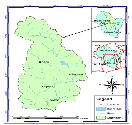
The White Volta Basin is one of the sub-basins of the Volta Basin and is located between latitudes 8°50' N to 14°05' N and longitudes 0°06' E to 2°50' W. The basin is bounded to the east by the Oti River Basin, to the west by the Black Volta River Basin and to the south by the Main/Lower Volta sub-basins. Burkina Faso and Ghana shares its northern and southern boundaries respectively. Figure 2.1 presents the map of the Volta Basin showing Volta White Basin and the six riparian countries.

The basin covers approximately 100,100 km2 at Nawuni and represents approximately 25% of the total Volta Basin. The drainage area in the Ghana part of the basin is approximately 50,000 km2_{and constitutes 44% of the total area of the White Volta Basin with the remaining part}

(5)

Kulpawn/Sissili rivers, take their sources in the central and north-eastern portions of Burkina Faso (WRC, 2008).

Located in the Guinea Savannah belt, the White Volta Basin’s ecology is typically Sahelian (hot and dry), with the vegetation consisting mostly of semi-arid grassland interspersed with short trees. Bush burning which is typically not controlled and causes enormous damage on the vegetation is rampant in the basin. It is usually used to induce rapid re-growth of rangeland, clear land for agricultural purposes, hunting, and creating fire belts at the onset of the dry season.

The basin has a uni-modal wet season which starts from April and peaks in August (Kwabena Kankam-Yeboah et al, 2013). The average annual rainfall of the basin is about 900 mm/annum. The basin is characterized by uniformly high temperatures throughout the year with a mean annual temperature of about 28 °C. The months of March and April are the hottest periods with a mean temperature of about 32 °C. August is the coolest month with a mean temperature of about 26°C. Generally, potential evapotranspiration in the Volta Basin is highest in the dry season where the availability of water is limited. However, actual evapotranspiration is lowest in the dry season and estimated at 2 mm/day and highest in the rainy season at 10 mm/day (Martin, 2005).

(6)

Figure 2.1 : Map showing the White Volta Basin, Volta Basin and the six riparian countries.

2.2 Data Overview

(7)

The quality of the raw water is monitored at least three times daily and at most twelve times daily.

Wagner et al., (2006) recommended that the estimation of suspended sediment concentration from turbidity measurements should be done by first comparing turbidity measured from a fixed-location to that of cross-section in-stream turbidity measurements. In this study, the GWCL abstraction point was considered as the fixed-location. The cross-section in-stream measurement were taken 50m upstream. The cross-section was divided into five equal widths and concomitant turbidity and water samples were taken using a Quanta Hydro lab Sonde and depth-integrated samplers respectively. The equal-width increment method of suspended sediment sampling (Gray et al., 2008) was employed using a DH-48 and DH-76 isokinetic depth-integrating sampler during low and high flows respectively. The cross-section turbidity measurements were also collected at three different depths (0.2, 0.6, 0.8 of total depth) as recommended by Anderson (2005). These measurements were then averaged to obtain mean daily in-stream turbidity and used in evaluating the representativeness of the data collected from fixed-location using a one-on-one plot.

The suspended sediment samples were collected from September 2012 to January 2014. As suspended sediment concentration in streams can change appreciably over seasonal timescales and during high flow events (Lawler et al., 2006) a gauge reader was engaged to take dip samples daily. Daily surface dip samples were taken concurrently alongside depth-integrated samples during monthly field visits. The surface dip samples were correlated with samples taken with the depth-integrated sampler to obtain a correction factor which was used to adjust the surface dip samples taken by the gauge readers (Akrasi, 2005).

The statistical parameters of the river discharge and SSC data are presented in Table 2-1.

Table 2-1: Statistical parameters of the river discharge, turbidity and SSC data at Nawuni

Variable Mean Sx Cv Csx Min Max

Max/Me an

Discharge (m3_/s)

429.2 6

414.8

0 0.97 1.66 40.8 1319.2 3.07

Turbidity (NTU)

322.6 6

219.1

8 0.68 0.97 93.0 1082.0 3.35

SSC (mg/l) 375.8

8

405.9

9 1.08 1.50 47.8 1908.0 5.08

(8)

From Table 2-1, it can be seen that the river discharge, turbidity and SSC data show a significantly low skewed distribution and this is confirmed by the low coefficient of variation and the ratio between the maximum and mean. These statistics potentially minimizes the variation of the model estimated SSC from the measured. Available suspended sediment concentration data for Nawuni were also obtained from the Water Research Institute, WRI of the Council for Scientific and Industrial Research, CSIR. The data which was part of measurements of suspended sediment concentrations of water samples collected from six rivers (Amisigo & Akrasi 1996) covers the period July 1994-March 1995. The surface dip sampling method was used in collecting the data at a sampling interval of 3 days on average. To correct for the underestimation of surface dip sampling, a correction factor of 25% was used to provide mean concentration values for the cross-section area (Akrasi, 2005). The 1994/95 suspended sediment concentration data was used to temporally validate the derived models.

2.3 Regression Analysis

The key elements for computing suspended sediment concentration (SSC) time-series data from periodic instantaneous SSC, turbidity, and streamflow data are the type and goodness-of-fit of the regression model used in the computation.

A simple linear regression (SLR) model relating turbidity to suspended-sediment concentration (SSC) is usually considered sufficient for reliable computations of SSC time-series. However, based on the criteria for determining the sufficiency of a SLR model, a multiple regression (MR) model relating both turbidity and streamflow to SSC could be employed to significantly improve the SLR model that is based on turbidity alone (Rasmussen et al., 2009).

In this study, the time-series (i.e. turbidity, stream and SSC) collected during the period September 2012 to December 2013 were used as the calibration data set. All the data sets were transformed using the base-10 logarithmic transformation. Transformation of the data sets prior to regression analysis makes the residuals more symmetric, linear, and homoscedastic (Rasmussen et al., 2009).

A SLR and MR models relating turbidity to SSC and turbidity and streamflow to SSC respectively were then developed and validated for the White Volta Basin. The models were validated with the 1994-1995 data sets. Diagnostic statistics were used to evaluate the performance of the derived models during the validation period. The appropriate model equation was selected and subsequently used to estimate long-term suspended sediment concentration and loads for the White Volta Basin.

(9)

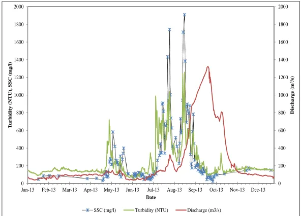
The relationship between the river discharge, suspended sediment concentration and turbidity at Nawuni in the White Volta was evaluated by plotting the time series of the 2013 calendar year. The plot was used to evaluate the variability of the turbidity and streamflow and their relationship with SSC in the White Volta Basin.

2.3.2 Evaluation of Fixed-Location and Cross-Section Turbidity

The development of the regression analysis was preceded by an evaluation of the relationship between the fixed-location turbidity as measured by GWCL and the in-stream turbidity as measured with the Quanta HydrolabSonde. Wagner et al., (2006) recommends that comparisons of fixed-location and cross-section in-stream turbidity measurements should be made part of the turbidity record analysis (Rasmussen et al., 2009). The relationship between the fixed-location turbidity and the in-stream turbidity was evaluated to check the representativeness of turbidity time-series as measured by GWCL. A plot of turbidity at the fixed-location and the in-stream turbidity was made and a one-on-one plot, i.e. y = x line was then drawn through the points on the plot.

2.3.3 Identification of Outliers

The development of the SSC regression model was also preceded by an evaluation of a scatterplot of the turbidity and SSC data. The scatter plot was used to identify possible outliers in the data set. The data was further examined by analyzing the residuals. Residuals that exceeded three standard deviations from the predicted line were considered insufficient for the regression analysis and therefore eliminated from the data set. . An extreme outlier is one for which the standardized residual is greater than three (3). The standardized residual is given by (Helsel and Hirsch, 2002): s i m i si h y y e    1 Eq.1

where yi and ym are the ith and mean of the response variable hi is the leverage and is given by:

   



     _n i m i m i i x x x x n h 1 2 2 1 Eq.2

where xi and xm are the ith and mean of the explanatory variable and n is the number of samples.

(10)



    n i m i n y y s 1 2 ) 2 ( ) ( Eq.3

2.3.4 Correlation Analysis

Correlation coefficients measure the strength of association between two variables (Helsel and Hirsch, 2002). The most commonly used measure of correlation is Pearson’s r which measures the linear association between two variables (Helsel and Hirsch, 2002) and is given by:



         _          n i y m i x m i S y y S x x n r 1 1 1 Eq.4

where n is the number of data points, xi and yi are the ith observation for the variables, xm and ym

are the means and Sx and Sy are the standard deviation of the variables. If the data lie exactly

along a straight line with positive slope, then r = 1 (Helsel and Hirsch, 2002). In this study, the relationship between explanatory and response variables was evaluated by computing the Pearson’s correlation coefficient and plotting the time series. The scatter plots and correlation coefficient helps to identify which variables are statistically related. Helsel and Hirsch (2002) suggest that before applying multiple linear regressions to any variables, it is important to understand the causes and consequences of multicollinearity. Multicollinearity is the condition where at least one explanatory variable is closely related to one or more other explanatory variables. In this study, variance inflation factor (VIF) was computed and used for measuring multicollinearity. The VIF is given by (Helsel and Hirsch (2002):



2



1 1 j j R VIF   Eq.5

where Rj2 is the coefficient of determination (R2) from a regression of the jth explanatory

variable on all of the other explanatory variables. In this study, VIF for turbidity and streamflow was computed by using the coefficient of determination (R2) from the regression of turbidity on stream flow.

2.3.5 Simple Linear Regression, SLR Analysis

After the correlation analysis, the SLR was used to establish a relationship between turbidity and SSC as a power function.

c aT

(11)

www.ijaer.in Copyright © IJAER 2016, All right reserved Page 814 SSC is the suspended sediment concentration (mg/l), and T is the turbidity (NTU), a and c are transport curve parameters (Gray and Simoes, 2008). Eq.6 was formulated as a linear model in base-10 logarithmic space to find a solution for transport-curve parameters.

The t-statistics, the p-value and the 90% confidence intervals were used to evaluate the performance of the SLR model. For a statistically significant linear relationship between turbidity and SSC, the absolute value of the t-statistics should be greater than 2 (Helsel and Hirsch (2002)).

The diagnostics statistics used to evaluate the SLR were the coefficient of determination adjusted (R2a) and the model standard percentage error (MSPE). The R2a for the turbidity indicates the

fraction of variability in the SSC that is explained by the model (Rasmussen et al., 2009). RMSE expressed as a percentage is referred to as the model standard percentage error (MSPE) (Rasmussen et al., 2009). For RMSE expressed in log-10 units, the MSPE interval is given by:

Upper 



10 1



100

RMSE

MSPE _and

Lower 



110



100

RMSE

MSPE _Eq.7

The MSPE and the 90% prediction intervals indicate the range in uncertainty associated with each regression-computed SSC value. SLR analysis is usually preferred where turbidity is the variable most strongly correlated with SSC or where MSPE is less than 20 percent (Rasmussen et al., 2009).

The SLR was further evaluated by examining the model residuals. Ordinary residuals are defined as the difference between the observed values and the model estimates (Moriasi et al., 2007). The residual error (ei) for the computed SSC values should be random and, in theory, should be

normally distributed with a mean of zero and a constant variance (Helsel and Hirsch, 2002). The residuals from a regression of SSC on the turbidity indicate how the model-estimated SSC varies from the observed SSC. A residual value of 0.00 indicates that the model-estimated SSC is equal to the observed value. A positive residual indicates that the observed value was larger than the estimated value, and a negative residual indicates that the observed value was less than the estimated value (Rasmussen et al., 2009). The variance of the residuals was evaluated by plotting them against the model estimated SSC.

2.3.6 Nonlinear Multiple Regression, NMR Analysis

(12)

0.025 (Rasmussen et al., 2009). A nonlinear multiple regression model was used to fit a 3rd order polynomial function of the form:

n w

n Q

b T c a

SSC log log

log    _Eq.8

where SSC is the suspended sediment concentration (mg/l), Qnw is streamflow (m3/s), T is the

turbidity (NTU), and a, bn, and c are transport curve parameters (Gray and Simoes, 2008). After

obtaining a solution, Eq. , was retransformed into a power function of the form:

c b

w T

aQ

SSC _Eq.9

The NMR was evaluated using the coefficient of determination (R2), sum of square errors (SSE).. The SSE estimates the total within-group noise using departures from the sample group mean. Error in this context refers not to a mistake, but to the inherent variability within a group (Helsel and Hirsch, 2002). The smaller the SSE, the better the model fits the sample with zero as the optimal best fit.

2.3.7 Bias Correction Factor, BCF

The derived regression equations were retransformed from the logarithmic space to linear space. This approach usually introduces a bias in the computed SSC (Rasmussen et al., 2009). The bias usually arises because regression estimates are the mean of the SSC for a given explanatory variable in logarithmic space, and retransformation of these estimates is not equal to the mean of the SSC for a given explanatory variable in linear space.

In this study, the nonparametric bias correction factor proposed by Duan (1983) was used to correct the bias due to the retransformation. The BCF is given by:

n BCF

n

i

e_i





 1

10

Eq.10

Where n is the number of samples, and eiis the residual or the difference between each measured

and estimated SSC, in log units.

2.4 Model Validation

(13)

to establish whether the model has the ability to predict the measured suspended sediment concentrations at Nawuni for a different time period.

The derived models were validated by comparing the model estimated SSC with measured daily suspended sediment concentration sampled from July 1994 to March 1995. The performances of the derived models were then evaluated using the coefficient of determination (R2), mean absolute error (MAE), percent bias (PBIAS) and the Nash-Sutcliffe efficiency (NSE).The R2 measures the degree to which two variables are linearly related and ranges from 0 to 1, with higher values indicating less error variance (Moriasi et al., 2007). MAE presents a more balanced perspective of the goodness-of-fit at average SSCs and range from 0 to +∞. A MAE value of 0 indicates a perfect fit (Kisi, 2007).The NSE on the other hand is a normalized statistic that determines the relative magnitude of the residual variance compared to the measured data variance and ranges from -∞ to 1.The optimal value of NSE is 1.0 (Moriasi et al., 2007). The R2, RMSE, MAE and NSE are respectively defined by:

        2 5 . 0 1 2 5 . 0 1 2 1 2                     _        _           N i mean i N i mean i N i mean i mean i P P O O P P O O R Eq.11       _ 



 N i i i P O N MAE 1 1 Eq. 12     _             



  N i mean i N i i i O O P O NSE 1 2 1 2 1 Eq.13

3. RESULTS AND DISCUSSIONS

3.1 Evaluating the relationship between Turbidity, Suspended Sediment Concentration and River Discharge

(14)

season and loose top soils from agricultural lands which are usually ploughed in May. The early rains however usually contribute insignificant runoff to the watershed outlet due to dry antecedent moisture conditions during that period. Additionally, bush burning, which damages vegetation, is rampant around this period in the basin and therefore presents little resistance to sediment transport into the river.

On the other hand, the figure also shows that while the turbidity and SSC peaks in late August, the streamflow peaks in late September. This can be attributed to the fact that, with increasing rainfall in the basin, the re-growth of the vegetative cover improves and provides resistance to sediment transport into the river. As runoff reaches its peaks, the basin becomes lush with vegetation thereby impeding the transport of sediments into the river. . This also implies that, the main source of sediments in the study area is mainly driven by upland erosion and sediment transport.

Figure 3-1: A plot of river discharge (m3/s), turbidity (NTU) and SSC (mg/l) at Nawuni for 2013

3.2 Relationship between Fixed-Location and Cross-Section Turbidity

Results of the evaluation of the relationship between the turbidity as measured at the fixed location by the GWCL and the mean cross-section turbidity measured with the Quanta Hydro lab Sondeis presented in Figure 3-2. The figure shows that the measured turbidity at the fixed-location overestimates the mean cross-section turbidity for the high turbidity values. This can be attributed to the fact that at high flows the flow velocities at the river banks are very low compared with that of the mid-section causing a semblance of laminar flow at the river bank.

0 200 400 600 800 1000 1200 1400 1600 1800 2000 0 200 400 600 800 1000 1200 1400 1600 1800 2000

Jan-13 Feb-13 Mar-13 Apr-13 May-13 Jun-13 Jul-13 Aug-13 Sep-13 Oct-13 Nov-13 Dec-13

Disc h ar ge (m 3/s) T u r b id ity (N T U) , S S C ( m g/l ) Date

(15)

The velocity gradient thus tends to force fine and other microbial materials to settle at the river banks resulting in high turbid waters compared to the mid-sections. The deviations from the 1:1 line are however minimal indicating a fairly harmonized data between the GWCL turbidity measurements at the fixed-location and the mean cross-section measurements by the Quanta Hydro lab Sonde.

Figure 3-2: Comparison of Turbidity from Fixed-Location (GWCL, Nawuni Headworks) and In-Stream Cross-Section Measurements (Quanta Hydrolab)

3.3 Identification of Outliers

Figure 3-3 presents the scatter plot of turbidity versus the suspended sediment concentration at Nawuni. In this study, no outlying data points were identified in a scatter plot of turbidity versus suspended sediment concentration consisting of all the time-series data used in the regression analysis. The standardized residuals were computed for the data and the maximum deviation from the predicted line found to be 2.14 which is less than the recommended value of 3. All the 99time-series data points were therefore considered sufficient for the regression analysis

y = 0.9264x + 1.1605 R² = 0.9651

0 100 200 300 400 500 600 700 800 900

T

u

r

b

id

ity

in

Cr

oss

-S

e

c

tion

(D

ata

fr

om

Qu

an

ta

Hyd

r

olab

)

Turbidity from Fixed-Location (Data from GWCL)

Y=X Plot

(16)

Figure 3-3: A scatter plot of turbidity (NTU) from GWCL and SSC(mg/l) 3.4 Correlation Analysis

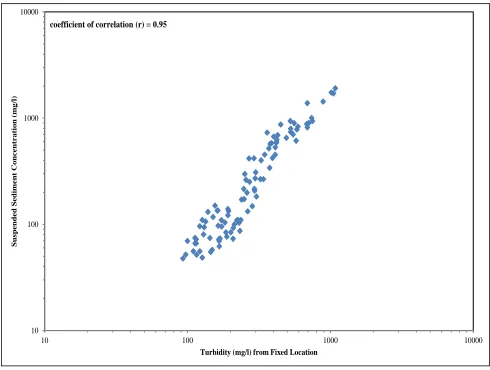
In this study, scatter plots and correlation coefficients in logarithmic space were used to evaluate the relationship between turbidity, streamflow and SSC. Figure3-4 presents a scatter plot of turbidity versus suspended sediment concentration in base-10 logarithmic transform space. The relationship shows a strong association with a correlation coefficient of 0.95.The plot showed a linear relationship between the turbidity and the SSC implying a linear regression model can be developed between them (Lee et al., 2009).

Figure 3-4: A plot of turbidity (NTU) and SSC mg/l) in log-10 space at Nawuni. 0

500 1000 1500 2000 2500

0 200 400 600 800 1000 1200

Su

spended

Sedim

ent

C

oncent

rat

ion

(m

g/

l)

Turbidity (mg/l) from Fixed Location

10 100 1000 10000

Su

spended

Sedim

ent

C

oncent

rat

ion

(m

g/

l)

(17)

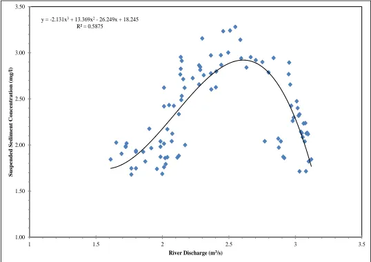
The relationship between the streamflow and SSC in log-10 transform space however shows a parabolic shape (Figure 3-5). An observation from Figure 3-1 and 3-5 shows that the SSC peaked in the 3rd week of August as streamflow just begins to rise. The plots also show that beyond this period, every incremental streamflow correspond with a decline in SSC. This period also concedes with the peak of the rainfall. As the soil moisture reaches saturation and the vegetative cover becomes lush, less sediment are being eroded from the uplands and transported to the watershed outlet.

With the cessation of rainfall in the basin, streamflow eventually decline in magnitude below the SSC. This suggests that the river remained turbid over a wide range of flows, and the suspended sediment concentrations remain relatively high during low flows. This relationship also implies that a nonlinear multiple regression model relating turbidity and streamflow to SSC would be applicable.

Figure 3-5: A plot of discharge (m3_{/s) and SSC (mg/l) in log-10 space at Nawuni.}

3.5 Regression Analysis

3.5.1 Simple Linear Regression Model (SLR)

Analysis of the regression residual plots for turbidity and SSC in linear space shows a heteroscedastic pattern (Figure 3-6). Heteroscedasticity occurs when the variability of the residuals increases as estimated SSC increase and suggests the need of variance stabilizing transformation of the response variable. In this study, the turbidity and SSC were therefore transformed using the base-10 logarithmic transform function.

y = -2.131x3+ 13.369x2- 26.249x + 18.245 R² = 0.5875

1.00 1.50 2.00 2.50 3.00 3.50

1 1.5 2 2.5 3 3.5

Su

spended

Sedim

ent

C

oncent

rat

ion

(m

g/

l)

(18)

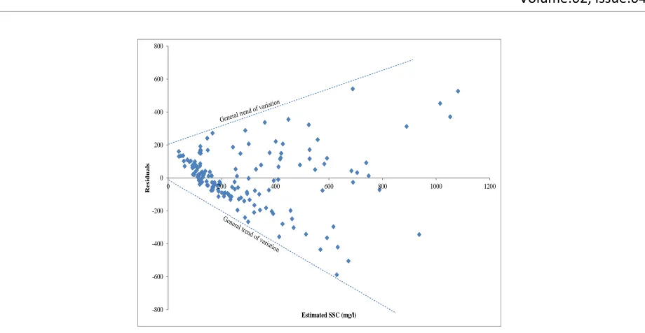
Figure 3-6: Computed suspended-sediment concentrations and regression residuals in linear space showing heteroscedasticity.

The residuals plot for the log-10-transformed regression however shows a homoscedastic pattern (i.e. constant variance) and is presented in Figure 3-7. The residuals were also evaluated for normality by plotting the residuals on a normal-probability plot (Figure 3-8) and computing the probability plot correlation coefficient (PPCC). According to Helsel and Hirsch (2002),the ideal transformation maximizes the probability plot correlation coefficient (PPCC) for the regression residuals and optimizes the normality of residuals. Non-normally distributed residuals will not be linear or equally distributed on a normal-probability plot and have a smaller PPCC(Rasmussen et al., 2009). From Figure 3-8, the probability plot for the log-10transformed regression shows a more linear, evenly distributed residuals and a high PPCC of 0.97.

Figure 3-7: Plot of computed suspended-sediment concentrations and regression residuals -800

-600 -400 -200 0 200 400 600 800

0 200 400 600 800 1000 1200

Re

sid

u

als

Estimated SSC (mg/l)

-0.8 -0.6 -0.4 -0.2 0 0.2 0.4 0.6 0.8

1 10 100 1000 10000

Re

sid

u

als

Estimated Suspended Sediment Concentration (mg/l)

(19)

Figure 3-8: Normal probability plot of the regression residuals

The SLR model in base-10 logarithmic space for the White Volta at Nawuni is given by:

.58 1 T 1.62log SSC

log₁₀  ₁₀ 

Eq. 14

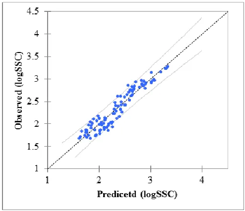
where SSC is the suspended-sediment concentration (mg/l) and T is the turbidity (NTU). Table 3-1 presents the model basic information, regression coefficients, and model diagnostic statistics. The best fit SLR model plot showing the 90% confidence interval is presented in Figure 3-9. The figure shows that given the significance level of 10%, the information brought by the explanatory variables is significantly better than what a basic mean would bring. Figure 3-10 also shows a plot of the predicted versus the observed SSC on a one-on-one plot in base-10 logarithmic space. The figure shows a uniformly distribution points around the one-on-one plot implying that the model did not significant over or underestimated the SSC.

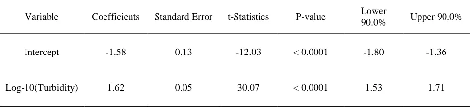
Table 3-1: SLR model coefficients and diagnostic statistics

Variable Coefficients Standard Error t-Statistics P-value Lower

90.0% Upper 90.0%

Intercept -1.58 0.13 -12.03 < 0.0001 -1.80 -1.36

Log-10(Turbidity) 1.62 0.05 30.07 < 0.0001 1.53 1.71

1 1.5 2 2.5 3 3.5

0 10 20 30 40 50 60 70 80 90 100

Re

sid

u

als

(20)

Figure 3-9: A plot of SLR of SSC and turbidity showing 90% confidence level for Nawuni (Sept. 2012-Dec. 2013)

(21)

The absolute values of the t-statistics of 12.03 and 30.07 for the intercept and turbidity respectively (Table 3-1), are greater than 2 and can be considered significant to be included in the SLR model. The p-values for the intercept and turbidity were all less than 0.0001 satisfying the null hypothesis at 90% confidence level. A standard error of 0.032 for the turbidity also shows less dispersion of the data around the regression line.

The diagnostics statistics used to evaluate the SLR model are also presented in Table 3-2. The coefficient of determination adjusted (R2a) for the turbidity indicates the fraction of variability in

the SSC that is explained by the model (Rasmussen et al., 2009). The R2a value of 0.902

indicates that the SLR model explains 90.2% of the variability in the SSC.

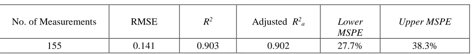
Table 3-2: SLR Model diagnostics for the White Volta Basin at Nawuni

No. of Measurements RMSE R2 _Adjusted_R2

a Lower

MSPE

Upper MSPE

155 0.141 0.903 0.902 27.7% 38.3%

The MSPE and the 90% prediction intervals indicate the range in uncertainty associated with each regression-computed SSC value. From Table 3-1, the 90-percent prediction interval was found to be 1.53 and 1.71 percent for the lower and upper significant levels respectively. This implies that, for every given turbidity value, there is a 90-percent certainty that the true SSC value occurs within 0.18 interval. The larger the 90-percent prediction interval, the more uncertainty there is associated with computed SSC (Rasmussen et al., 2009).

According to Rasmussen et al., (2009) SLR analysis is preferred for sites where turbidity is the measure most strongly correlated with SSC or where MSPE is less than 20%. From Table 3-2, the Upper and Lower MSPE were found to be 38.3% and 27.7% respectively which are greater than the recommended 20%. This implies that, an additional explanatory variable such as the river discharge may improve the estimation of SSC in a multiple linear regression model.

The bias correction factor (BCF) was estimated using Eq.10 and found to be 0.027. Applying the BCF and retransforming Eq.14, the final SLR model for the White Volta Basin at Nawuni on the basis of turbidity and SSC is given by:

62 . 1

027 . 0 T

SSC _{Eq. 15}

where SSC is the suspended-sediment concentration (mg/l) and T is the turbidity (NTU).

(22)

The MSPE for the SLR model for the White Volta at Nawuni was found to be greater than 20% indicating that an additional explanatory variable such as streamflow in a NMR model may improve the model estimation of SSC.

In this study, the applicability of the NMR was initially analyzed by computing the variance inflation factor (VIF) for turbidity and streamflow using the coefficient of determination (R2) from the regression of turbidity on streamflow. The R2_{was found to be 0.014 resulting in a VIF}

of 1.00 which is considered ideal for the development of a NMR model. A VIF of 1.00 suggest that turbidity and streamflow are not strongly multi collinear and could be used as explanatory variables in a multiple model to compute SSC.

The NMR model in base-10 logarithmic space relating turbidity and streamflow to SSC for the White Volta is given by:

3 2 log 09 . 0 log 42 . 0 log 25 . 0 log 49 . 1 73 . 1 log w w w Q Q Q T SSC       Eq.16

The NMR model equation in base-10 logarithmic space shows a linear relationship between turbidity and SSC and a polynomial relationship between the streamflow and SSC as confirmed in the correlation analysis.

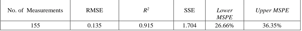
The diagnostics statistics used to evaluate the NMR model are presented in Table 3-3. The R2 value of 0.915 indicates that the NMR model explains 91.5% of the variability in the SSC. The sum of square errors (SSE) was found to be 1.704 indicating that the model estimated SSC did not significantly depart from the measured mean and hence a very good fit.

Table 3-3: NMR Model diagnostics for the White Volta Basin at Nawuni

No. of Measurements RMSE R2 _SSE _Lower

MSPE

Upper MSPE

155 0.135 0.915 1.704 26.66% 36.35%

The upper and lower MSPE for the NMR were found to be 36.35 and 26.66% respectively which are greater than the recommended 20%. This implies that, the additional explanatory variable, the streamflow, may not sufficiently improve the estimation of SSC by the NMR model.

(23)

. 1 30 . 0

010 .

0 Q

T

SSC



w _Eq.17

where SSC is the suspended-sediment concentration (mg/l), Qw is the river discharge (m3/s) and

T is the turbidity (NTU).The low magnitude of the streamflow exponent (<1) implies that SSC in the White Volta tends to decrease during rising streamflow.

A plot of the NMR model predicted versus the observed SSC in base-10 logarithmic space is presented in Figure 3-11. The figure shows a uniformly distribution points around the one-on-one plot implying that the model did not significant over or underestimated the SSC.

Figure 3-11: Comparison of NMR model predicted versus observed SSC at Nawuni (Sept. 2012-Dec. 2013)

3.6 Model Validation

(24)

Table 3-4: Model Performance Statistics for the SLR and NMR of the White Volta Basin for the validation period

Model Type R2 _MAE _NSE

SLR 0.93 3.29 0.93

NMR 0.79 1.65 0.66

Figure 3-12: Comparison of Observed and Model Estimated SSC (mg/l) for the White Volta at Nawuni

The coefficient of determination, R2_{was found to be 0.93 and 0.79 for the SLR and the NMR}

models respectively. This indicates that the turbidity alone explains the variability of the SSC in the White Volta Basin than a combination of turbidity and streamflow. Figure 3-12 shows a plot of predicted SSC versus observed SSC on a one-on-one plot. For a perfect estimate, the data fitting a function should fall along the 1:1 line, where the model estimates are equal to the observed. The plot shows that both the SLR and NMR predicted very well the observed SSC at Nawuni during the validation period. The NMR model however tends to overestimate the high SSC in the basin. The model efficiencies and mean absolute errors were also found to be very good with values of 0.93 and 3.29 for the SLR and 0.66 and 1.65 for the NMR respectively.

Overall, the performance statistics indicates that the SLR model can be considered the better option for estimating long-term time series of SSC for the White Volta Basin. The addition of

0 100 200 300 400 500 600 700 800

Model

E

st

im

at

ed

SS

C

(

m

g/

l)

Observed SSC (mg/l)

(25)

streamflow as an explanatory variable in the MLR did not improve the estimation of the SSC and this is reflected in the magnitude of the streamflow exponent.

Based on the above results, it is evident that monitoring turbidity in conjunction with limited sediment sampling will provide a reasonable surrogate method for estimating SSC on a daily or sub-daily time scale. The derived SLR model was subsequently used to estimate long-term time series of sediment loads in the White Volta Basin.

3.7 Estimation of Suspended Sediment Load (SSL) for the White Volta Basin

The SLR model was used to estimate SSC based on long-term turbidity data obtained from the Ghana Water Company Ltd. Long-term sediment loads were subsequently computed using Eq. 15 (Horowitz, 2003):

SSC

Q

SSL



0 .

0864



_w



Eq.18

where SSL is the daily sediment load (metric tonnes/day), 0.0864 is a conversion factor, Qw is

the streamflow (m3/s) and SSC is the suspended sediment concentration (mg/l).Using Eq. 18, the daily sediment loads of the White Volta Basin at the Nawuni hydrological station was computed based on the estimated SSC and streamflow. Monthly and annual sediment loads were also computed. A plot of the long-term monthly computed SSL is presented in Figure 3-13.

Figure 3-13: Long term monthly computed SSL (tonnes/day) for the White Volta Basin at Nawuni

(26)

White Volta was then computed from the daily loads and found to be 5.68x106_{metric tonnes per}

annum which is consistent with results obtained by Akrasi (2005).Milliman et al., (1992) also estimated the mean annual suspended sediment load of the Volta Basin to be 19x106metric tonnes per annum. This result is significantly low compared with the 127x106 metric tonnes/yr of sediment loads generated in the Blue Nile (El Monshidet al., 1997).

4. CONCLUSION

The collection of suspended-sediment data in the White Volta Basin in particular and the Volta Basin in general has been sporadic and at best project/program demand driven. In this study, the use of the surrogate method of estimating long-term suspended-sediment data using turbidity and streamflow was examined.

Continuous turbidity data collected by GWCL as part of their water quality requirement was calibrated with measured SSC data and used to compute long-term time series of suspended sediment load for the White Volta Basin at Nawuni. A simple linear regression model between turbidity and the measured SSC data was derived.

With the challenge of developing sustainable and continuous SSC sampling due to lack of resources, sediment rating curves based on continuously monitored turbidity by GWCL provides a better option of computing long-term suspended-sediment loads in the country. The developed sediment rating curves can be bi-annually updated with detailed sampling of SSC. Based on the analysis of the SLR and NMR models, the simple-linear regression, SLR model was selected for the study area on the basis of the relationship between the base-10 logarithmic transformation of turbidity and SSC.

The mean annual suspended sediment load for the White Volta Basin at Nawuni is estimated to be 5.68x106 metric tonnes per annum. Although the sediment load obtained in this study is seen as relatively low compared with other rivers, the results provide a valuable basis for assessing the potential sedimentation of the Volta Lake.

REFERENCES

Akrasi, S. A., 2005. The assessment of suspended sediment inputs to Volta Lake. Lakes & Reservoirs: Research and Management 10: 179–186.

(27)

Andah, Winston E.I. (ed.) 2005. Volta River Basin: Enhancing Agricultural Water Productivity Through Strategic Research. Technical Report No. 8, Challenge Program on Water and Food, P.O. Box 2075, Colombo, Sri Lanka

Anderson, C.W., 2005, Turbidity: U.S. Geological Survey Techniques of Water-Resources Investigations, book 9, chaps. A6.7, http://pubs.water.usgs.gov/twri9A.

Arino, Olivier; Ramos Perez, Jose Julio; Kalogirou, Vasileios; Bontemps, Sophie; Defourny, Pierre; Van Bogaert, Eric, 2012. Global Land Cover Map for 2009 (GlobCover 2009).© European Space Agency (ESA) & Universitécatholique de Louvain (UCL), doi:10.1594/PANGAEA.787668.

Asselman, N.E.M., 2000. Fitting and Interpretation of Sediment Rating Curves.Journal of Hydrology, 234, pp.228-248.

Coyne etBellier, 1993. White Volta Development Scheme – Prefeasibility Study.Volta River Authority. Chapter 2.

Duan, Naihua, 1983, Smearing estimate-A nonparametric retransformation method: Journal of the American Statistical Association, v. 78, no. 383, p. 605–610.

Edwards, T. K., and Glysson, G. D., 1999. Field Methods for Measurement of Fluvial Sediments. In: U.S. Geological Survey Techniques of Water-Resources Investigations, Book 3, Chapter C2, U.S. Geological Survey, Information Services, Reston, Virginia.

El Monshid, B. E. F., El Awad, O. M. A. and Ahmed, S. E., 1997 " Environmental effect of the Blue Nile Sediment on reservoirs and Irrigation Canals" , Int. 5th Nile 2002 Conf., Addis Ababa, Ethiopia.

Gray, J.R., Glysson, G.D., and Edwards, T.E., 2008, Suspended-sediment samplers and sampling methods, in Garcia, Marcelo, ed., Sedimentation engineering—Processes, measurements, modeling, and practice: American Society of Civil Engineers Manual 110, chap. 5.3, p. 320–339.

(28)

Helsel, D.R., and Hirsch, R.M., 2002, Statistical methods in water resources—hydrologic analysis and interpretation: U.S. Geological Survey Techniques of Water-Resources Investigations, book 4, chap. A3, 510,http://pubs.usgs.gov/twri/twri4a3/.

Khanchoul, K., Benslama, M., and Remini, B., 2010.Regressions on Monthly Stream Discharge to Predict Sediment Inflow to a Reservoir in Algeria. Journal of Geography and Geology, Vol. 2, No.1; pp.36 – 47.

Kisi, Özgür, 2007. Development of Stream flow-Suspended Sediment Rating Curve Using a Range Dependent Neural Network. International Journal of Science & Technology Volume 2, No 1, 49-61.

Kwabena Kankam-Yeboah, Emmanuel Obuobie, Barnabas Amisigo & Yaw Opoku-Ankomah (2013) Impact of climate change on stream flow in selected river basins in Ghana, Hydrological Sciences Journal, 58:4, 773-788, DOI: 10.1080/02626667.2013.782101

Lane, L. J., Hernandez, M., and Nichols, M., 1997.Processes Controlling Sediment Yield from Watersheds as functions of Spatial Scale, Environmental Modelling and Software, Vol.12, No.4, pp.355 - 369.

Lewis, Jack, 1996, Turbidity controlled suspended sediment sampling for runoff event load estimation: Water Resources Research, v. 32, no. 7, p. 2,299–2,310.

Milliman, J. D., and J P M Syvitski, 1992. Geomorphic/Tectonic Control of Sediment Discharge to the Ocean : The Importance of Small Mountainous Rivers', The Journal of Geology 100, 525-544.

Moriasi, D. N., Arnold, J. G., Liew, M. W. V., Bingner, R. L., Harmel, R. D., and Veith, T. L. 2007. Model Evaluation Guidelines for Systematic Quantification of Accuracy in Watershed Simulations, T. ASABE, 50, 885–900.

Nichols, M. H., 2006. Measured Sediment Yield Rates from Semiarid Rangeland Watersheds. Rangeland Ecology & Management, 59(1), pp.55-62.

(29)

Rasmussen, P.P., Gray, J.R., Glysson, G.D., and Ziegler, A.C., 2009, Guidelines and procedures for computing time-series suspended-sediment concentrations and loads from in-stream turbidity-sensor and streamflow data: U.S. Geological Survey Techniques and Methods, book 3, chap. C4, 52 p.

Schmengler, A. C., 2011. Modeling soil erosion and reservoir sedimentation at hillslope and catchment scale in semi-arid Burkina Faso. University of Bonn, PhD Dissertation,

http://hss.ulb.uni-bonn.de/diss_online.

Verstraeten, G., and Poesen, J., 2001. Factors controlling sediment yield from small intensively cultivated catchments in a temperate humid climate. Geomorphology, 40, pp.123–144.

Wagner, R.J., Boulger, R.W., Jr., Oblinger, C.J., and Smith, B.A., 2006, Guidelines and standard procedures for continuous water-quality monitors—station operation, record computation, and data reporting: U.S. Geological Survey Techniques and Methods 1–D3, 51 p., 8. http://pubs.water.usgs.gov/tm1d3.

Walling D. E. & Webb B. W. (1983) Patterns of sediment yield. In: Background to Palaeohydrology (ed. K. J. Gregory) pp. 69–100. Wiley, Chichester.