Inventory Cost Analysis Work in Process (Wip) Under Focus of Lean Accounting, Simulation and Optimization Scenarios

(1)

DOI:10.31142/etj/v4i3.01, I.F. - 4.449

© 2019, ETJ

545 Diana F. Guerrero-González

1

, ETJ Volume 04 Issue 03 March 2019

Inventory Cost Analysis Work in Process (WIP) Under Focus of Lean

Accounting, Simulation and Optimization Scenarios

Diana F. Guerrero-González

1

, José Alfredo Jiménez-García

2

, Salvador Hernández-González

3

, Edgar Augusto

Ruelas-Santoyo

4

, Moisés Tapia-Esquivias

5

, Vicente Figueroa-Fernández

6

1,2,3,5,6_{Department of Industrial Engineer, Tecnológico Nacional de México en Celaya} 4_{Department of Industrial Engineer, Tecnológico Nacional de México en Irapuato}

ABSTRACT: In this research, we present a cost analysis of the materials that are in a queue to be processed, better known as work-in-process inventory (WIP, for its acronym in English).

The inventory in process will be analyzed with three models: 1. A system of waiting lines, 2. Lean Accounting and 3. Simulation of discrete events that helps measure the benefits of Lean Accounting, applying an objective function to determine the minimum cost of WIP. This was obtained by applying a key tool called Simrunner. A cost breakdown structure was also established at each stage of the process. The present work is of interest to the administrators and managers of the Lean team and useful for short-term decision making.

KEYWORDS: value stream costs, simulation, work in process inventory, waiting for lines, promodel

I. INTRODUCTION

In the 21st century, global competition is forcing all companies to be much more efficient to stay in the market. This is how the reduction of costs and waste becomes a critical element for organizations that seek to stay and follow the vanguard [1]. The philosophies to reduce waste and costs is Lean Manufacturing which, together with Lean Accounting, will allow managing challenges related to costs and delivery level with great success. Within these wastes are inventories of work in process (WIP) that increase costs per area, can become obsolete and process flexibility is lost. Within these wastes are WIP that increase costs per area, can become obsolete and process flexibility is lost.

[2] mentions that estimated costs are relevant inputs for decision-making models and therefore it is important that they are estimated appropriately. In the case of WIP and waiting times, the Lean Accounting methodology is applied. Despite the great potential of the Lean strategies, many studies report flaws in the final results [3], which is why an interaction of Lean tools, optimization, and simulation is proposed.

In this research, it is proposed to develop scenarios of discrete events simulation created in Promodel in which the processes and effects of these are identified in detail by calculating performance measures. Value stream costing analysis is applied, a lean accounting tool to analyze the WIP related costs. Optimization is also applied through simulated models in Promodel. Simrunner will provide scenarios that minimize costs, both the cost of waiting time

for entities in the locations and the inventory of work in process.

II. METHODOLOGY

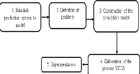
Figure 1 shows the steps developed to analyze the behavior and costs of the WIP. Under the assumption that their Lean manufacturing methods have reached a state of sufficient maturity. The methodology proposed by the author.

Figure 1.Steps for the development of the investigation.

III.RESULTS

1.Establish production system to model

(2)

546 Diana F. Guerrero-González

1

, ETJ Volume 04 Issue 03 March 2019

A production system is selected where metal parts are manufactured, which are classified into 5 categories, each category with a different monthly demand. The production process consists of 4 stations (A, B, C and D. Station A works with 3 machines, B 3 machines, C 1 machine and D with 3 machines.

The production rate per hour in a type A machine is 2 units. Type B of 2 units.Type C of 4 units and D of 2 units per hour. One month of 20 days and 8 daily hours of work, exponential times are assumed.

2. Definition of the problem

The problem is to measure the financial and operational aspects in the simulated system to determine the level of service that minimizes the total cost of the system without affecting the outputs of the finished product. The measurement is based on:

1. Jackson's open network. 2. Lean Accounting tool. 3. Optimization with Simrunner.

3. Construction of the simulation model

The basic stages for the development of a simulation model are described, describing in detail what must be done in each of these steps to warrant the success of a simulation project.

For this purpose, the suggestions of [5], [6] and [7] are considered.

A. Data collection

For the development of this stage, data are obtained from [8], [9] and [4] for the construction of the simulated model. Jackson's open network in Promodel, which according to the system represented in Figure 2 above, defines the following data in Table 1 and 2, also defining the process routes:

TABLE 2.MONTHLY DEMAND BY TYPE OF PIECE AND ROUTES OF THE PROCESS.

B. Verification of the model

Verification of the simulation model. The behavior of the input variables was visually inspected to verify their proper functioning and to validate that the parameters used in the system description work correctly.

C. Validation of the model

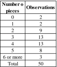
This process consists of carrying out a series of tests with the actual input information described in the data collection to ratify their behavior and analyze their results. In this case, the behavior of the arrivals to the real system is analyzed, which is defined in historical data that the pieces arrive at station C with a Poisson distribution, at an average rate λ = 3.01.

To reformulate the arrival process, a random sample is taken by counting the number of pieces that arrive at the inspection station, the grouped data are shown in table 3.

From the parameter defined for the data, the hypotheses to be tested are proposed:

Ho: Poisson (λ =3)

H1: Another type of distribution

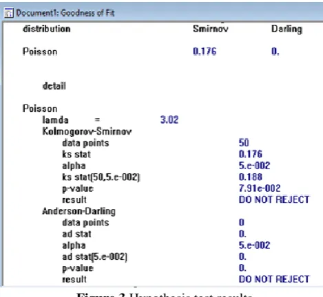
Hypothesis tests are performed by applying Stat: Fit with a significance level of α = 0.05 shown in Figure 3. H0 is not rejected, the data behave according to a Poisson distribution close to λ = 3.01.

Type

piece a

Type

piece b

Type

piece c

Type

piece d

Type

piece e

Demand

68

409

272

136 Routes

A,B,C

A,B,D

B,D

A,C

B,C

Figure 2. Systemnetwork.

Node

λ (number of arrivals per unit

of time)

μ (number of services per unit

of time)

S (number of servers)

ρ (condition of non-saturation)

A 4.68 2 3 0.78

B 5.55 2 3 0.95

C 3.01 4 1 0.75

D 4.21 2 3 0.7

TABLE 1.SIMULATED SYSTEM DATA

0 2

1 2

2 9

3 13

4 13

5 8

6 or more 3

Total 50

Number o

pieces Observations

(3)

547 Diana F. Guerrero-González

1

, ETJ Volume 04 Issue 03 March 2019

Figure 3.Hypothesis test results.

4.VSCA of the process

When validating the simulation model. the results obtained by Promodel are extracted, such as cycle time, WIP, total of pieces produced, the waiting time, etc., facilitating the analysis of value flow costs.

The cost of the value flow is generally calculated weekly and takes into account all costs in the value stream. No distinction is made between direct and indirect costs. All the costs of the value chain are considered direct. In this case, WIP costs and operating costs are included.

Define the value flow

Following the methodology proposed in the flow of value, the operations of the system, times and their jobs for the current situation are shown in table 4.

To define the flow of value, a monthly period is chosen, assuming that a daily shift of 8 hours is worked from Monday to Friday (1 month = 20 days x 8 hours by day).

Analyze capacity

Table 5 shows the operational analyzes with the most important performance measures to be controlled [10] which were calculated with Promodel.

Table 6A) and B) shows the total costs of the value chain for the current month, in the process that totals the amount of 18939.78 dollars extracted from [10]. Because not all the pieces go through the same process, a value flow costing is performed for each piece taking as a reference the process route shown above in figure 2.

TABLE 6. B) VALUE FLOW COSTS (VSC) OF THE CURRENT SITUATION OF THE PROCESS.

The calculation of the average cost for each type of piece is obtained by dividing the total cost (dollars) of the value chain by the number of units produced.

• Average cost per unit for piece a

• Average cost per unit for piece b

• Average cost per unit forpiece c

• Average cost per unit for piece d

• Average cost per unit for piece e =

Introduction of income accounts by value chain

Table 7 shows the unit price of sale for each type of piece. Typically, to calculate the unit sale price, 85% of the average cost per unit is added [11].

Node A 106606.0122 487250 1877078 Node B 157092.7133 487250 38465.9 2045939 Node C 52508.009 194900 1358338 Node D 162606.6292 487250 1914368 Total 478813.3637 1656650 38465.9 7195723

Machinery costs ($)

Other costs

Total costs Value flow

cost

Operation costs ($)

TABLE 4.OPERATION AND NUMBER OF WORKERS IN THE PRODUCTION SYSTEM.

Estation A Cut Exponential 30 2

Estation B Polished Exponential 30 2

Estation C Painting Exponential 15 1

Estation D Print Exponential 30 2

Total 105 7

Process Time (min)

(per machine)

Number of workers Descripción

Type piece a 9592.01 65 60 12

Type piece b 9590.53 400 368 48

Type piece c 9587.78 266 249 30

Type piece d 9588.34 265 260 20

Type piece e 9590.68 132 123 20

Total 47949.34 1128 1060 130

Operational summary Cycle time

(min)

Number of pieces entered into the system per month

Productivity (units by

month)

WIP TABLE 5.CURRENT OPERATIONAL SUMMARY.

Node A 935520 155920 155920 35861.6

Node B 935520 155920 155920 115770.6

Node C 935520 77960 58470 38980

Node D 935520 155920 155920 17151.2

Total 3742080 545720 526230 207763.4

Value flow cost

Material costs ($)

Workforce costs ($)

Costos de amortización

($)

Amortization costs ($) TABLE 6.A)VALUE FLOW COSTS (VSC) OF THE CURRENT SITUATION OF THE PROCESS.

Piece

Price ($)

Type a

162841.6786

Type b

29345.3134

Type c

29423.8581

Type d

23021.0033

Type e

51202.3739

Unit price of sale

(4)

548 Diana F. Guerrero-González

1

, ETJ Volume 04 Issue 03 March 2019

In this stage, the company's results accounts will be developed by value chains, as shown in table 8 A)toE).

TABLE 8. A)INCOME STATEMENT BY VALUE CHAIN.

TABLE 8. B)INCOME STATEMENT BY VALUE CHAIN.

TABLE 8. C)INCOME STATEMENT BY VALUE CHAIN.

TABLE 8. D)INCOME STATEMENT BY VALUE CHAIN.

TABLE 8. E)INCOME STATEMENT BY VALUE CHAIN.

Simulate capacity uses

In this stage, the VSCA will be introduced to evaluate the process in financial terms. For this purpose, the information corresponding to the time dedicated to productive activities and times dedicated to non-productive activities is calculated for each position. In this case, in Table 9 and 10 work stations, A and B respectively are analyzed.

Sales 9770500.716 9770500.7

Cost of materials 2806560 2806560

Personnel cost 389800 389800

Amortization cost 370310 370310

WIP cost 190612.2 190612.2

Cost of operation 316206.7345 316206.73

Profit / loss of the value stream 5697011.782 5697011.8

General expenses 116425.85

Plant benefits 5580585.9

Manufacturing flow of value 1

($)

Total plant ($) Type of piece a

Sales 10799075.33 10799075

WIP cost 168783.4 168783.4

Profit / loss of the value stream 6461906.577 6461906.6

Plant benefits 6345480.7

Manufacturing flow of value 1 ($)

Total plant ($) Type of piece b

Sales 7326540.667 7326541

WIP cost 132921.8 132921.8

Profit / loss of the value stream 4379199.524 4379200

Plant benefits 4262774

Total plant ($) Type of piece c

Sales 5985460.858 5985461

WIP cost 74841.6 74841.6

Cost of operation 159114.0212 159114 Profit / loss of the value stream 3432195.237 3432195

General expenses 77960

Total plant ($) Type of piece d

Sales 6297891.99 6297892

WIP cost 154750.6 154751

Cost of operation 209600.7223 209601

Profit / loss of the value stream 3614230.667 3614231

General expenses 116426

Manufacturing flow of value 1

($)

Total plant ($) Type of piece e

Piece

Price ($)

Type a

162841.6786

Type b

29345.3134

Type c

29423.8581

Type d

23021.0033

Type e

51202.3739

(5)

549 Diana F. Guerrero-González

1

, ETJ Volume 04 Issue 03 March 2019

TABLE 9) PRODUCTION CAPACITY ANALYSIS, NON

-PRODUCTIVE AND AVAILABLE FROM WORK STATION A.

TABLE 10) PRODUCTION CAPACITY ANALYSIS, NON -PRODUCTIVE AND AVAILABLE FROM WORK STATION B.

In later stages, the future state of the capacity analysis will be presented, expecting an increase in the production of units. Therefore, a reduction in the average cost of each piece produced.

After carrying out the cost analysis by implementing the VSCA tool, we proceed to calculate the minimum cost of the WIP of the production system simulated in Promodel. the processing times and inter-arrival times of the different types of piece are taken as a restriction to meet the demand to reduce the WIP.

5. Experimentation

Once the costs under the Lean Accounting approach were analyzed, they were used for optimization purposes and thus meet the objectives set in the research.

The cost of making the sub-assemblies wait in the row within the objective function shown in equations 1 to 4 is taken as a response variable. The objective is to find the service rate and the time between arrivals of the entities that minimizes the cost total of the value stream chain.

MIN CT = (C1* fila a maximum contents) (1) MIN CT = (C1* fila b maximum contents) (2) MIN CT = (C1* fila c maximum contents) (3) MIN CT = (C1* fila d maximum contents) (4)

C1: Cost to keep the WIP in the system.

Queue maximum contents: Maximum number of WIP in the course of simulation.

CT: Total cost of the process.

The restrictions or decision variables for the problem are identified as follows:

137 ≤ X1 ≤ 145 19 ≤ X2 ≤ 24 31 ≤ X3 ≤ 36 66 ≤ X4 ≤ 71 5 ≤ X5 ≤ 30 10 ≤ X6 ≤ 15

X1: Time between arrivals of piece a - queue a X2: Inter-arrival time of part b - queue a X3: Inter-arrival time of part c and d - queue b X4: Inter-arrival time of part e - queue a X5: Processing time in station A, B and D X6: Processing time in station C

Optimization

Execution of 25 experiments in the Simrunner optimization module, resulting in the best solution for experiment 10. Table 11 shows the suggestions that Simrunner makes to reduce the inventory of work in process and its costs both for WIP and for the times of process.

TABLE 11) VARIABLES FOR THE SIMULATED PRODUCTION SYSTEM PROPOSED BY SIMRUNNER.

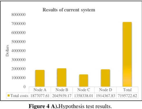
In figure4 A) y B) it can be seen that with the suggestion provided by Simrunner subtracting the total cost of figure4 A) minus the total cost of figure4 B) a reduction of 134568.705 dollars pesos per month is obtained.

Figure 4 A).Hypothesis test results.

Productive Manufacturing 688 28770.88 2 3

Not

productive Repairs - - -

-Productive max 76.12 - - -Non-productive 23.88 - -

-Actual state

Number of operators

Number of machines Activity Quantity

(units)

Cycle time

Productive Manufacturing ₈₀₀ ₃₈₃₆₁ ₂ ₃

Not

productive Repairs - - -

-Productive max 84.25% - -

-Non-productive 15.75% - -

-Activity Quantity (units)

Cycle time (min)

Number of operators

Number of machines

Actual state

Variable

Arrives piece a - queue a

Arrives piece b - queue a

Arrives piece c y d - queue a y b

Arrives piece e - queue b

Process times C

Process times A, B and D

71

13

25 Process times and inter-arrival times of the entities to the

system proposed by simrunner

Exponential times

140

22

34

Node A Node B Node C Node D Total Total costs 1877077.61 2045939.17 1358338.01 1914367.83 7195722.62

0 1000000 2000000 3000000 4000000 5000000 6000000 7000000 8000000

D

ol

la

rs

(6)

550 Diana F. Guerrero-González

1

, ETJ Volume 04 Issue 03 March 2019

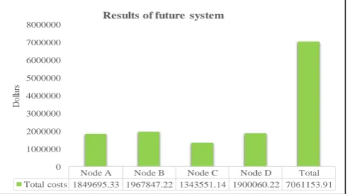
Figure 4 B).Hypothesis test results.

Simulation model was run for both lines with the data proposed by simrunner to observe the behavior of the average cost per unit and to verify that there is an improvement in the process. Because the operation times reduce their costs, they also generate less work inventory in process and increasing the total of pieces produced and completed of 97.62% in the demand.

Figure 5 A) to E) shows the reduction in the average cost for the types of pieces.

Figure 5 A).Reduction of current average cost against future average cost.

Figure 5 B).Reduction of current average cost against future average cost.

Figure 5 C).Reduction of current average cost against future average cost.

Figure 5 D).Reduction of current average cost against future average cost.

Figure 5 E).Reduction of current average cost against future average cost.

IV.CONCLUSIONS

The interaction of Lean tools, simulation and optimization applied in this cost analysis allowed to describe in a detailed and practical way the behavior of the work inventory in process and the waiting time for the production system simulated in Promodel mentioned in the description of the problem. Costs involved in the flow of value, were obtained by simplifying its method so that it was understood by the Lean team responsible and said costs were monitored over time without losing sight of the stated objective.

Simulating the model allowed building a system to carry out the optimization purposes that facilitated knowing the current and future state of the costs related to the flow of value and being able to make short-term decisions.

The value flow cost analysis shows that the best work option for the simulated system is to reduce the variables of the process time and time between arrivals in each of the stations. Minimizing the total cost of the value chain $ 6904.5 pesos per month equivalent to $ 82854 pesos per year. It is important to mention that the evolutionary algorithms that were applied to find the minimum solution in Simrunner, is a good estimate, but not the optimal one.

Calculating again the average costs for each type of piece, a reduction is observed in this, thus proving an improvement in the process and satisfying the demand an average 97.62%.

It is important to mention that the evolutionary algorithms that were applied to find the minimum solution in Simrunner, is a good estimate, but not the optimal one. Node A Node B Node C Node D Total

Total costs 1849695.33 1967847.22 1343551.14 1900060.22 7061153.91 0 1000000 2000000 3000000 4000000 5000000 6000000 7000000 8000000 D ol la rs

Results of future system

88022.4921 79401.2855 9.79 0 20000 40000 60000 80000 100000

Average cost per unit Average cost per unit % Reduction

Current system Future system

D

o

ll

ars

Type piece a

15862.3263 14013.6998 11.65 0 5000 10000 15000 20000

D

o

ll

ars

Type piece b

15904.8145 14378.7475 9.59 0 5000 10000 15000 20000

D

o

ll

ars

Type piece c

12443.7803 _11915.0166 4.24 0 2000 4000 6000 8000 10000 12000 14000

Average cost per unit Average cost per unit % Reduction Current system Future system

D

o

ll

a

rs

Type piece d

27676.9694 25472.2606 7.96 0 5000 10000 15000 20000 25000 30000

D

o

ll

ars

(7)

551 Diana F. Guerrero-González

1

, ETJ Volume 04 Issue 03 March 2019

As future work we propose the application of this methodology to a real-world company, of the mechanical metal branch.

REFERENCES

1. Cerón, J., Madrid, J., & Gamboa, A. (2015). Desarrollo y casos de aplicación lean manufacturing. Magazin Empresarial Economia & Empresa, 11(28), 23-44.

2. Vrat, P. (2014). Materials managment an integrated systems approach. India: Springer.

3. Karim, A., & Urif-Uz-Zaman, K. (2013). A methodology for effective implementation of lean strategies and its performance evaluation in manufacturing organizations. Business process management, 9(1), 169-196.

4. Cabrera, M. (2009). Trabajo de grado Manual de prácticas de simulación de sistemas discretos con Promodel. Bogota.

5. García, E., García, H., & Cárdenas, L. (2006). Simulación y análisis de sistemas con promodel.México: Pearson.

6. Harrell, C., Ghosh , B., & Bowden, R. (2003). Simulation using promodel. New York: Mc Graw Hill.

7. Render, B., Stair, R. J., & Hanna, M. (2009). Quantitative analysis for management. Upper saddle river: Prentice hall.

8. Hillier, F., & Lieberman, G. (2001). Introduction to operation research. New York: Mc Graw Hill. 9. Taha, H. (2007). Operations research an

introduction. New Jersey: Pearson.

10. Maskell, B., Baggaley, B., & Grasso, L. (2011). Practical lean accounting: a proven system for measuring and managing the lean enterprise. New York: Taylor & Francis.