Error Estimation Using Fuzzy Linear Regression Analysis

Vol. 13, No. 1, 2017, 69-76

ISSN: 2320 –3242 (P), 2320 –3250 (online) Published on 22 September 2017

www.researchmathsci.org

DOI: http://dx.doi.org/10.22457/ijfma.v13n1a7

69

International Journal of

Error Estimation Using Fuzzy Linear Regression

Analysis

S.Ismail Mohideen1, A.Nagoor Gani2 and U.Abuthahir3

1

PG & Research Department of Mathematics, Jamal Mohamed College (Autonomous) Tiruchirappalli-620020, Tamil Nadu, India. E-mail: [email protected]

2

PG & Research Department of Mathematics, Jamal Mohamed College (Autonomous) Tiruchirappalli-620020, Tamil Nadu, India. E-mail: [email protected]

3

PG & Research Department of Mathematics, Jamal Mohamed College (Autonomous) Tiruchirappalli-620020, Tamil Nadu, India. E-mail: [email protected]

Received 7 September 2017; accepted 20 September 2017

Abstract. In this paper an attempt is made to reduce the error of non-fuzzy data using fuzzy linear regression. A numerical example has been analyzed. It is concluded from the example that the normal regression method is better compared to fuzzy linear regression method.

Keywords: Linear regression, symmetric triangular fuzzy number and fuzzy regression.

AMS Mathematics Subject Classification (2010): 03E72, 62J05, 62J12

1. Introduction

Regression analysis, including statistical regression analysis and fuzzy regression analysis, aims to determine the best-fit model for describing the functional relationship between dependent variables and independent variables by exploiting the knowledge from the given input-output data pairs. Some discrepancy between the observed values (from the data sets) and the estimated values (from a regression model) can occur due to measurement errors and/or modeling errors.

Regression analysis is one of the areas in which fuzzy set theory is used frequently, since Tanaka [4] initiated research on fuzzy linear regression (FLR) analysis. This area is widely developed and wide varieties of methods are proposed. One approach to deal with FLR is Linear Programming (LP). This approach was first introduced by Tanaka and developed by others, and next approach is least squares method, which was first introduced by Celmins [1] and developed by others [2].

The fuzzy set theory introduced by Zadeh [5] has derived meaningful applications in many field of studies. The idea of fuzzy set is welcomed because it handles uncertainty and vagueness. In fuzzy set theory, the membership of an element of a fuzzy set is a single value between zero and one.

70

for all given input–output data sets. Here, the basic idea is to minimize the fuzziness of the model by minimizing the total support of the fuzzy coefficients, subject to all data.

The rest of this chapter is organized as follows: In Section 2, the basic concept and definitions are presented. In Section 3, fuzzy linear model is given. In Section 4, fuzzy regression analysis is given and finally numerical example is given In Section 5.

2. Preliminaries

Definition 2.1. A fuzzy set (FS) is defined by = { x, (x) : x∈ A , (x) ∈ [0,1] }. In the pair (x, (x)), the first element x belong to the classical set A and the second element belong to the interval [0, 1] is called membership function.

Definition 2.2. A fuzzy set is convex if

(λ + (1- λ) ) ≥ Min ((), ( )),∀, ∈ R and λ∈[0,1].

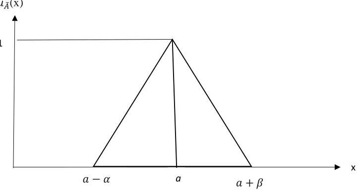
Definition 2.3. A triangular fuzzy number (TFN) with left spread and right spread is denoted by and corresponding membership function is given,

(x) =

()

∈ [ − , ]

∈ [, + ]

0 "ℎ$%&'$

(

where a∈R; , β>. The symbolic representation of TFN is _*+, = [a:, β]. Here and β

are called left and right spreads of membership function (x) respectively The diagrammatic representation of a TFN is as following

Figure 1: Triangular fuzzy number

Definition 2.4. A Linear Programming Problem (LPP) is defined as:

Maximize z= c x Subject to Ax = b, x≥ 0

x (x)

a

− ₊

71

where c = ( -, - _,… , -_/), b = (00 , … , 0₁)* and A= [₂₃]_1×/where all the parameters are crisp.

2.5. Graded mean integration representation method-defuzzification

If A~ = (, , ₅) is a triangular fuzzy number then the graded mean integration representation of A~ is given by 678 = [+ 4 + ₅] 6⁄

3. Fuzzy linear regression model (FLR)

Fuzzy functions and fuzzy linear models [3] are presented, here for continuation. The general form of FR model is given by

=> = f(x, ) = _? + + + … + _// (1) where => is the fuzzy output, ₂ , i= 1,2,…,n is an fuzzy coefficient and X = (, _,… , _/) is an n dimensional non-fuzzy input vector. Each Triangular Fuzzy Number (TFN) coefficient ₂ can be defined by _*+,= [a; ₂, ₂] where₂, ₂are called the left and right spreads of membership function (x) respectively. When two spreads are equal, the TFN is known as symmetric triangular fuzzy number (STFN). Hence a TFN _*+, = [a;,

β] is said to be STFN if = (say m), this concept gives the definition of STFN as follows:

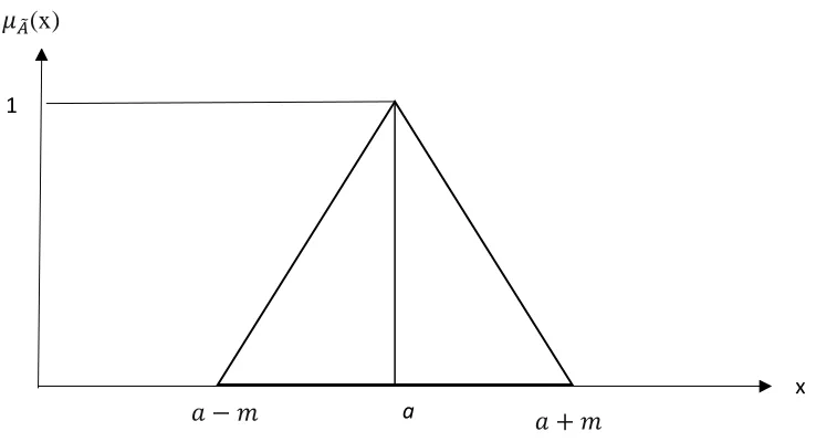
A fuzzy set in R is said to be a STFN if there exist real number a and m where m>0 such that the membership functions are derived from Figure 2.

Figure 2: Symmetric triangular fuzzy number

(x) =

(1)

1 ∈ [ − @, ]

1

1 ∈ [, + @]

0 "ℎ$%&'$

(

x (x)

a

− @ _{+ @}

72

STFN can be represented as _A*+, = [a; @,@], where a is the center, @ is the spread of membership function (x).

The fuzzy components are assumed to be STFNs. The fuzzy output from the linear model f(x, ) in (1) can be expressed as =>=f(x, ) = ( B(), C())where B() is the center of the of linear model f(x, ) and has the formB() = _?+ + ⋯ +

// and C()is the spreads of membership functions of f(x, ).

C_{() = @?+ @⃓ ⃓ + ⋯ + @/ ⃓ /⃓}

Then the membership of => defined in (1) can be represented as,

(y)=

F G

HI[(J∑ (1L JL∑ 1L)(1L L|J∑ 1L|)L L|L|)] = ∈ [(?+ ∑ 2 22) − (@?+ ∑ @2 2|2|), (?+ ∑ 2 22)] [(J∑ L LL)(1J∑ 1L L|L|)]I

(1J∑ 1L L|L|) = ∈ [(?+ ∑ 2 22), (?+ ∑ 2 22)+ (@?+ ∑ @2 2|2|)] 0 "ℎ$%&'$

(

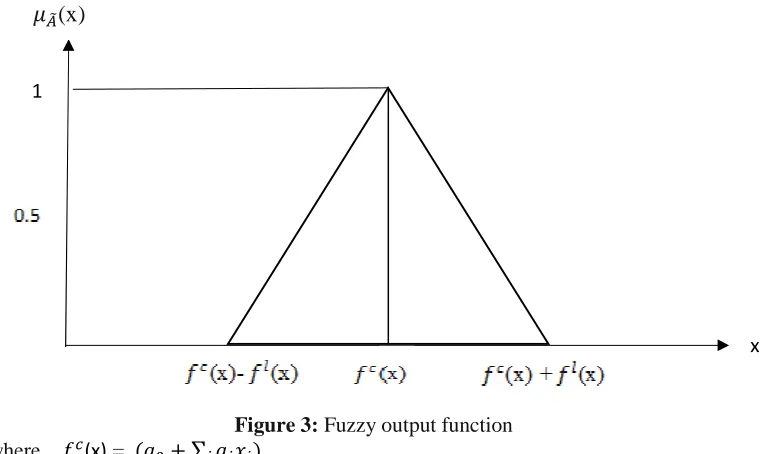
The diagramatic representation of fuzzy output function of an FN with h-level set is presented in the following figure.

Figure 3: Fuzzy output function where B(x) = (_?+ ∑ _{2 22})

B_(x)-C_{(x) =(?+ ∑ 2 22) − (@?+ ∑ @2 2|2|)} B_(x)+C_{(x) =(?+ ∑ 2 22) + (@?+ ∑ @2 2|2|)}

4. Analysis of fuzzy linear regression

The objective of the Fuzzy Linear Regression (FLR) method with non-fuzzy data is to determine the parameters such that the fuzzy output set {=₃} is associated with (=₃) ≥

h where h∈[0,1] and ‘h’ is chosen for the purpose of generating the best-fitting model. Now, the problem is to minimize the fuzziness of the output. Since, the values of the membership function of the fuzzy output are the function of the spread of the membership function, minimizing the spread of the membership function and hence it leads to the minimization of the fuzziness of the output.

x (x)

73

Minimize z = Min {C()} where C()is defined in (2) Minimize z = Min {C()} = Min {(@_?+ ∑ @/_{2O 2}∑ N1_{3O 3}N} (3) Subject to the set of constraints =₃∈ [f(₃)]h,

where [f(₃)]h = [_?]h + []h₃+ [ ]h₃+ . . . + [_/]h₃ such that [..]h denotes the h-level set of an Fuzzy Number. By using the fuzzy membership function for the output, the two constraints of the FLR model are given by

I[(J∑ L LL)(1J∑ 1L L|L|)]

(1J∑ 1L L|L|) ≥ ℎ (4)

and

[(J∑ L LL)(1J∑ 1L L|L|)]I

(1J∑ 1L L|L|) ≥ ℎ (5)

Simplifying (4) and (5), we have

= − [(?+ ∑ 2 22) − (@?+ ∑ @2 2|2|)] ≥ ℎ(@?+ ∑ @2 2|2|) (6) and

[(?+ ∑ 2 22) + (@?+ ∑ @2 2|2|)] − = ≥ ℎ(@?+ ∑ @2 2|2|) (7) Again simplifying, we get

(?+ ∑ 2 22) − (1 − ℎ)(@?+ ∑ @2 2|2|) ≤ = (8)

and [(_?+ ∑ _{2 22}) + (1 − ℎ)(@_?+ ∑ @_{2 2}|₂|)] ≥ = (9) Therefore, the problem is reduced to the following form:

Minimize z = Min {C()}

Min {C()} = Min {@_?+ ∑ @/_{2O 2}∑ N1_{3O 3}N} and

Subject to the constraints (8),(9) and @_? ≥0 and ₂, @₂ ≥0 for i=1,2,…,n

By using the software TORA, the values of the center and spread of membership can be estimated. This gives the FN coefficients as follows:

? = [_?;@_?, @_?]

= [;@, @]

⁞

/ = [_/;@_/, @_/]

By using the values of _?, …… _/ the FLR model becomes

=> = _? + + + … + _//

The value of => can be estimated by substituting the values of , …. _/, the estimated values of =>are actually STFNs which can be defuzzified to crisp number by using the function principle

A = [+ 4 + ₅] 6⁄ (10)

5. Numerical illustration

Numerical problem is considered with the value of h = 0.7

Example 5.1. Consider the values for X and Y in the following table to calculate the coefficients of the FLR model for i=1

j 1 2 3 4 5 6

3 1 2 4 6 7 8

74 Let us consider the value of h = 0.7 Minimize z = Min {C()}

Min {C()} = Min {(@_?+ @∑ NS_{3O 3}N)} Subject to the constraints

? + ₃ + 0.3@_? + 0.3@₃≥y[from (9)]

? + ₃ - 0.3@_? - 0.3@₃≤y [from (8)]

where ₃ represents the component of x in the jth entry value. The number of functional constraints depend on the number of data sets available. From the example six different sets of values (x, y) will generate 12 functional constraints respectively. Substituting the given values, the LPP becomes,

Min {C()} = Minimize {@_?+ 28 @ } Subject to the constraints

? + 1 + 0.3@_? + 0.3@≥3010

? + 1 - 0.3@_? - 0.3@ ≤3010

? + 2 + 0.3@_? + 0.6 @≥4500

? + 2 - 0.3@_? - 0.6 @≤4500

? + 4 + 0.3@_? + 1.2 @≥4400

? + 4 - 0.3@_? - 1.2 @≤4400

? + 6+ 0.3@_?+ 1.8 @≥5400

? + 6 - 0.3@_?- 1.8 @ ≤5400

? + 7 + 0.3@_? + 2.1 @≥7295

? + 7 - 0.3@? - 2.1 @ ≤7295

? + 8 + 0.3@_? + 2.4 @ ≥8195

? + 8 - 0.3@_? –2.4@ ≥8195 where _?, , @_?, @≥0.

By using the software Tora, the estimated values of the center and spread of membership function is given by

?= 2486.6667, = 615.8333, @_?= 2605.5556, @= 0.

where the minimized value of the objective function on the spread is Min {C()} = Minimize {@_?+ 28 @ }= 2605.5556

Now the FN coefficients are as follows:

? = [2486.6667; 2605.5556, 2605.5556]

= [615.8333; 0, 0] The FLR model is given by

=> = _? +

=>= [2486.6667; 2605.55,2605.55]+[615.8333; 0, 0](1)

=> = [3102.4997;2605.55,2605.55]

The transformed crisp value of => is given by

Y = [+ 4 + ₅] 6⁄ = [3102.4997 + 4(2605.55) + 2605.55] /6 Y = 2688.3805

The next value of Y can be calculated here, => = _? +

=>= [2486.6667; 2605.55,2605.55]+ [615.833; 0, 0] (2)

75 The transformed crisp value of => is given by

Y = [+ 4 + ₅] 6⁄ = [3718.3333 + 4(2605.55)+ 2605.55] /6 = 2791.0188 Similarly, the other values of Y are estimated and are presented in the following table

3 Observed =₃ =Y_X $₃= =Y − =_{X 3} $₃

1 3010 2688.381 -321.619 103438.7812

2 4500 2791.018 -1708.98 2920619.476

4 4400 2996.297 -1403.7 1970382.112

6 5400 3201.57 -2198.43 4833094.465

7 7295 3304.21 -3990.79 15926404.82

8 8195 3406.85 -4788.15 22926380.42

48680320.08

Table 1

5.1. Determination of error using ordinary regression method

The linear regression equation is Y = a + b X (A)

The value of a and b can be determined by using the following normal equation. ∑ Z + b∑ Z = ∑ Z[(B)

n a + b∑ Z = ∑ [ (C) The values of X and Y becomes,

X Y \] \^

1 3010 1 3010 2 4500 4 9000 4 4400 16 17600 6 5400 36 32400 7 7295 49 51065 8 8195 64 65560 28 32800 170 178635

Table 2

From (C) ⇒ 6a + 28b = 32800 From (B) ⇒28a + 170b = 178635

Solving (B) and (C) we have, a = 2433.1356 and b = 650.0423

Therefore the regression model (A) becomes, Ŷ = 2433.1356+ 650.0423X The other values of Y are estimated and are presented in the following table

3 Observed =₃ =Y_X $₃= =Y − =_{X 3} $₃

1 3010 3083.1779 73.1779 5355.005048

2 4500 3733.2202 -766.78 587951.2617

4 4400 5033.3048 633.3048 401074.9697

6 5400 6333.3894 933.3894 871215.772

7 7295 6983.4317 -311.568 97074.80556

8 8195 7633.474 -561.526 315311.4487

2277983.263

76 6. Conclusion

In this paper, fuzzy linear regression with symmetrical triangular number is used for prediction of values instead of normal linear regression. Error values is also found out for both fuzzy linear regression and normal linear regression. The error value of normal regression analysis is efficient than that of fuzzy linear regression from the above example.

REFERENCES

1. A.Celmins, A least squares model fitting to fuzzy vector data, Fuzzy Sets and Systems, 22 (1987 245-269.

2. H.Hassanpour, H.R.Maleki and M.A.Yaghoobi, Fuzz linear regression model with crisp coefficients: A goal programming approach, Iranian Journal of Fuzzy System, 7 (2) (2010)19-39.

3. R.Parvathi, C.Malathi, M.Akram and K.T.Atanassov, Intuitionistic fuzzy linear regression analysis, Fuzzy Optimization and Decision Making, 12(2) (2012) 215-229. 4. H.Tanakaand H.Lee, Interval regression analysis by quadratic programming