Volume 32 - Article 16 | Pages 487–532

(1)

DEMOGRAPHIC RESEARCH

VOLUME 32, ARTICLE 16, PAGES 487−532

PUBLISHED 18 FEBRUARY 2015

http://www.demographic-research.org/Volumes/Vol32/16/ DOI: 10.4054/DemRes.2015.32.16

Research Article

Urban fertility responses to local government

programs: Evidence from the 1923 – 1932 U.S.

Jonathan Fox

Mikko Myrskylä

©2015 Jonathan Fox & Mikko Myrskylä.

This open-access work is published under the terms of the Creative Commons Attribution NonCommercial License 2.0 Germany, which permits use, reproduction & distribution in any medium for non-commercial purposes, provided the original author(s) and source are given credit.

(2)

1 Introduction 488 1.1 Historical U.S. fertility declines and a 1920s acceleration 489

1.2 A 1920s fertility story 491

2 Public programs and changes in fertility 494

2.1 Conservation of child life 494

2.2 Charity for children and mothers & outdoor care of poor 496

3 Measuring local fertility 497

4 U.S. municipal fertility, 1920 – 1932 497

5 Data 500

6 Model and estimation 503

7 Conclusion 512

8 Acknowledgements 513

References 514

Appendices 519

A Alternative measures of municipal fertility rates 519

B Additional sensitivity analyses 522

B.1 Including city-specific trends 522

B.2 Including state-specific trends 523

B.3 Distributed lags 523

B.4 Arellano-Bond Dynamic Panel Model 524

(3)

Urban fertility responses to local government programs:

Evidence from the 1923 – 1932 U.S.

Jonathan Fox1

Mikko Myrskylä2

Abstract

BACKGROUND

During the 1920s and early 1930s, U.S. fertility declined overall but with large regional variations. Changes in foreign born populations explain only part of this. Differences in public health and poverty relief programs may further help explain these declines because of their potential impact on fertility determinants, in particular on breastfeeding and child mortality.

OBJECTIVE

We investigate whether public health investments in child health (conservation of child life programs) and poverty relief (outdoor care of poor or charity for children and mothers) affected fertility for U.S. cities over 100,000 persons between 1923 and 1932.

METHODS

We analyze data covering 64 cities between 1923–1932 that include birth information from the U.S. Birth, Stillbirth and Infant Mortality Statistics volumes and city financial information from the Financial Statistics of Cities volumes. Time and city fixed-effects models are used to identify the impact of public investments on fertility.

RESULTS

Fixed effects estimates indicating the conservation of child life programs explain about 10 % of the fertility change between 1923 and 1932. Outdoor care of poor did not seem to be related to fertility. Investments in charity for children and mothers were associated with fertility increases, possibly because poorer areas experienced relative increases in both higher fertility and charitable spending.

CONCLUSIONS

Public spending on child health was strongly related to decreasing fertility in the U.S. during the 1920s, possibly because of increased breastfeeding and decreased child

1_{Freie Universität Berlin, Germany. E-Mail: [email protected].} 2

(4)

mortality. This leads to a better understanding of the 1920s fertility decline and highlights how public policy may affect fertility.

1. Introduction

During the 1920s and early 1930s, before the enactment of the New Deal, fertility in large American urban areas trended downward, with the Total Fertility Rate (TFR) dipping below modern day replacement levels (about 2.3) likely for the first time.3 While fertility across large urban areas declined on average, cities varied in their fertility trajectories. There is no consensus as to what caused this variation, but in this paper we present empirical evidence showing that at least part of the variation in fertility outcomes across the large U.S. municipalities during the 1920s and early 1930s was due to differences in municipal investments in child health education and poverty relief programs. While there were no public programs explicitly targeting fertility, the conservation of child life programs during the 1920s may have reduced fertility indirectly by educating individuals about behaviors and methods to reduce infant mortality. Additionally, charitable programs were implemented across municipalities as a way to alleviate the harmful effects of poverty. By changing the family incentives for children, these may have also affected fertility.

Determining a relationship between the public investments and fertility is relevant both for understanding the 1920s–1930s declines in U.S. fertility rates as well as for informing current policy. While the child health programs were not implemented with the explicit intent of lowering fertility, the programs advocated the importance of birth spacing and smaller families for improvements in child health outcomes (Woodbury 1925, Lathrop 1919). A relationship between the child health programs and fertility would indicate that people altered their behavior in response to the programs. Thus, the conservation of child life programs may have had consequences beyond their stated goals. As the child health programs were implemented in a period of distress over falling birth rates (Newmayer 1911; Meckel 1990, pp. 102), and, as indicated by Margaret Sanger, “contraceptive information has been classed with obscenity, pornography and abortion” (Sanger 1931), it is likely the programs veered away from explicit discussion of fertility. However, improvements in child mortality are closely related to fertility, so the baby-saving campaigns may have also translated to fewer births in the first place. Determining whether these programs affected fertility will shed

3_{TFR estimates for each census between 1800 and 1990 for the white population of the U.S. are available in}

(5)

light on why the decline in urban fertility rates accelerated in the 1920s, and also on why fertility varied so much across U.S. cities. Regional variation in fertility has been a constant feature of the United States, and continues to be the case today (U.S. Bureau of the Census 2011: Section 2, Table 82). Understanding how investment in different types of public programs can influence fertility illustrates how conscious policy can lead to differences in fertility rates across otherwise similar areas.

1.1 Historical U.S. fertility declines and a 1920s acceleration

U.S. fertility was declining from at least as early as the mid to late 1800s. Some have dated the beginning of American fertility decline to the start of the 19th century (Hirschman 1994, David and Sanderson 1987), others arguing that the decline began in 1840 and that a broad reduction in marital fertility was not seen until the post-civil war period (Hacker 2003). The decline stopped in the late 1930s (U.S. Bureau of the Census 1975).

The reasons offered for the decline focus on changing demographic, religious, or economic circumstances. We do not attempt a full explanation of the different factors driving the fertility declines, instead we briefly overview some of the more important explanations to then determine their applicability to the 1920s. For a more complete overview, see Guinnane (2011).

(6)

cost of raising a surviving child (Barro and Becker 1989), potentially increasing fertility.

The above factors have limited power in explaining the acceleration of fertility decline in the 1920s, which is illustrated in Figure 1. This figure plots birth rates for women aged 15 and 44 between 1909 and 1950, and shows a clear acceleration in fertility decline in the 1920s. This decline accelerated in the urban areas as well. For cities over 100,000 persons, the ratio of children aged under 1 to women aged 15 to 44 declined from 75/1000 in 1910, to 72/1000 in 1920, and 57/1000 in 1930. Many of the explanations that work for earlier periods do not fit urban areas in the 1920s. First, there were no recessions – in urban areas, individuals were better off relative to the 1910s. Second, the proportion of married women between the ages of 15 and 44 increased from 60.5% in 1920 to 60.9% in 1930, and the singulate mean age at marriage declined from 22.7 in 1920 to 21.2 in 1930. Proximate factors such as fertility control and mortality decline remain candidate explanations accelerating fertility decline, but these may not be the whole story and we do not know what the ultimate factors behind these are.

Figure 1: Native white fertility trends, 1909 to 1950

Notes: Source is Series B5-10 in the Historical Statistics of the United States, Colonial Times to 1970.

0 20 40 60 80 100 120 140

B

ir

th

R

at

e

f

o

r

W

o

m

e

n

a

ge

d

1

5

t

o

4

Year

(7)

1.2 A 1920s fertility story

The mystery of the 1920s fertility decline was first addressed by Richard Easterlin in 1961, and he argues that the decline was driven by a changing population composition; reductions in fertility among the foreign born and rural populations caused fertility to decline (Easterlin 1961). Changes in immigrant demographics, specifically the shift of immigrants from eastern and southern European countries to immigrants from western and northern European countries, changes in the foreign-born sex ratio, and an aging of the female foreign-born population reduced foreign-born fertility. Easterlin attributed one-third of the decline in total white fertility in the 1920s to the reduction in the fertility of the foreign-born white population (Easterlin 1961, pg. 878). It was for these reasons, Easterlin argues, that U.S. fertility declined in the relatively prosperous 1920s. However, while this may explain much of the overall trend of fertility in the U. S., it does less to explain why the fertility decline accelerated in the large urban areas of America. Rural-to-urban migration is unlikely to drive down urban fertility rates. And while some areas in the U.S. did have large foreign born populations, such as New York and Connecticut with over 26 percent of the state populations having been born overseas in 1920, many areas did not. Despite the tendency of the foreign born to concentrate in large urban areas, many cities over 100,000 persons in 1920 had foreign born populations under 20 percent. For these areas, changes in the foreign born population would not fully explain declining fertility.

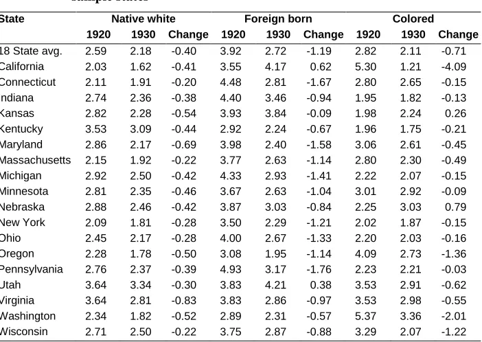
We analyzed the contribution of a changing foreign-born population to changes in state-level fertility over 1920–1930. Table 1 separates state level fertility changes by the population groups “Native white,” “Foreign born white,” and “Colored,” for states that were part of the 1920 Birth Registration Area (BRA) and had at least one city over 100,000 persons in 1920. Colored includes Asians, Pacific Islanders, Hispanics and other minority groups.4 Table 1 shows the almost universal decline in fertility across all population groups. In every state for which the calculations are possible, native white fertility declined between 1920 and 1930. With the exception of Kansas and Nebraska, this was also true for fertility among the colored population.

4_{”Colored” includes different populations for different states. For California, Oregon, and Washington,}

(8)

Table 1: Total fertility rate by population group in 1920 and 1930 BRA sample states

State Native white Foreign born Colored 1920 1930 Change 1920 1930 Change 1920 1930 Change 18 State avg. 2.59 2.18 -0.40 3.92 2.72 -1.19 2.82 2.11 -0.71 California 2.03 1.62 -0.41 3.55 4.17 0.62 5.30 1.21 -4.09 Connecticut 2.11 1.91 -0.20 4.48 2.81 -1.67 2.80 2.65 -0.15 Indiana 2.74 2.36 -0.38 4.40 3.46 -0.94 1.95 1.82 -0.13 Kansas 2.82 2.28 -0.54 3.93 3.84 -0.09 1.98 2.24 0.26 Kentucky 3.53 3.09 -0.44 2.92 2.24 -0.67 1.96 1.75 -0.21 Maryland 2.86 2.17 -0.69 3.98 2.40 -1.58 3.06 2.61 -0.45 Massachusetts 2.15 1.92 -0.22 3.77 2.63 -1.14 2.80 2.30 -0.49 Michigan 2.92 2.50 -0.42 4.33 2.93 -1.41 2.22 2.07 -0.15 Minnesota 2.81 2.35 -0.46 3.67 2.63 -1.04 3.01 2.92 -0.09 Nebraska 2.88 2.46 -0.42 3.87 3.03 -0.84 2.25 3.03 0.79 New York 2.09 1.81 -0.28 3.50 2.29 -1.21 2.02 1.87 -0.15 Ohio 2.45 2.17 -0.28 4.00 2.67 -1.33 2.20 2.03 -0.16 Oregon 2.28 1.78 -0.50 3.08 1.95 -1.14 4.09 2.73 -1.36 Pennsylvania 2.76 2.37 -0.39 4.93 3.17 -1.76 2.23 2.21 -0.03 Utah 3.64 3.34 -0.30 3.83 4.21 0.38 3.53 2.91 -0.62 Virginia 3.64 2.81 -0.83 3.83 2.86 -0.97 3.53 2.98 -0.55 Washington 2.34 1.82 -0.52 2.89 2.31 -0.57 5.37 3.36 -2.01 Wisconsin 2.71 2.50 -0.22 3.75 2.87 -0.88 3.29 2.07 -1.22

Notes: The “Total Fertility Rate” is the sum of the age specific fertility rates for 5 year age groups for women between 15 and 44. “Colored” includes Black, Asian, American Indian, and other minorities. For 1930, this category also includes “Mexican”. Mexican births were severely underreported in 1930 and likely also in 1920. In 1920, Mexicans were generally enumerated under “White,” however in 1930 they began to be enumerated under “Other.” The large difference in the California TFR for the group of “Other” results from this under reporting and change in enumeration.

(9)

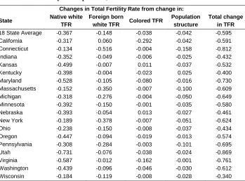
Connecticut. However, in most cases the relative population proportions and age structure did not account for a large proportion of the fertility decline. In half of the states (Indiana, Kansas, Kentucky, Maryland, Nebraska, Oregon, Utah, Virginia, and Washington), changes in native white fertility accounted for over 70 percent of the decline, while in another four (Wisconsin, Ohio, Minnesota, and California) it constituted over 50 percent. The analysis above does not account for rural versus urban fertility, so for those areas with large rural populations this may still be consistent with the Easterlin story. However, Table 2 indicates that it was fertility reductions within the population groups, not compositional changes, which drove the fertility decline in Birth Registration Areas during the 1920s.

Table 2: Fertility decomposition, 1920–1930

Changes in Total Fertility Rate from change in:

State Native white TFR

Foreign born

white TFR Colored TFR

Population structure

Total change in TFR 18 State Average -0.367 -0.148 -0.038 -0.042 -0.595 California -0.317 0.060 -0.292 -0.042 -0.591 Connecticut -0.134 -0.516 -0.004 -0.158 -0.812 Indiana -0.352 -0.049 -0.006 -0.025 -0.432 Kansas -0.499 -0.007 0.011 -0.037 -0.532 Kentucky -0.398 -0.004 -0.023 0.025 -0.400 Maryland -0.528 -0.105 -0.080 -0.016 -0.730 Massachusetts -0.152 -0.350 -0.007 -0.100 -0.609 Michigan -0.318 -0.276 -0.004 -0.050 -0.649 Minnesota -0.392 -0.150 -0.001 -0.035 -0.580 Nebraska -0.393 -0.054 0.013 -0.027 -0.461 New York -0.189 -0.378 -0.007 -0.051 -0.624 Ohio -0.238 -0.150 -0.008 -0.037 -0.434 Oregon -0.447 -0.094 -0.019 -0.013 -0.574 Pennsylvania -0.308 -0.284 -0.003 -0.101 -0.695 Utah -0.731 -0.076 -0.038 -0.024 -0.869 Virginia -0.587 -0.012 -0.162 -0.001 -0.761 Washington -0.439 -0.096 -0.046 -0.030 -0.612 Wisconsin -0.184 -0.119 -0.008 -0.028 -0.340

Notes: TFR stands for “Total Fertility Rate,” or the sum of the age specific fertility rates for 5 year age groups for women between 15 and 44.

(10)

2. Public programs and changes in fertility

Compositional changes explain only a part of the 1920s’ urban fertility decline; other factors need to be considered. Changing behaviors, values, and a response to economic incentives have been shown to be important in other periods, and may be responsible for some of the fertility change during the 1920s. We look at the interaction of these topics with local government programs, which has not been considered before. We evaluate whether local government programs, implemented to improve health and welfare, influenced fertility. Their role is important for any telling of a 1920s fertility story, despite these programs not explicitly targeting fertility.

Although there has been much work in the economics and demographic literature to understand how individuals make fertility decisions and how fertility trends have evolved over time, less work has been done to understand the relationship between U.S. government programs and local fertility. One exception finds that New Deal relief positively influenced fertility (Fishback, Haines, and Kantor 2007). Other work has looked at this relationship in developing countries and found, for instance, that cash transfers in Honduras increased fertility, but there was no distinguishable effect for similar programs in Mexico and Nicaragua (Stecklov et al. 2007).

During the 1920s there existed no large scale federal relief programs. Prior to the New Deal, poverty relief, public health, and other public goods were distributed at the state, municipal, and county levels. We focus on three different municipal level public programs – conservation of child life and its emphasis on public health education, charity for children and mothers, and outdoor care of poor – to examine whether investments in these influenced fertility across cities.

2.1 Conservation of child life

(11)

departments also had programs to inspect school children, where physicians or nurses conducted annual examinations and identified medical issues. In a few cities, smallpox vaccinations were given during these examinations, but more commonly the inspection was conducted and any defects found were referred to a private physician. Infant welfare stations were also set up in many of the different cities. Activities at these infant welfare stations varied considerably, but generally consisted of the supervision of expectant mothers and new infants, lectures, baby shows, and distribution of free literature (U.S. Public Health Service 1923).

Table 3: Health department budget expenses for conservation of child life

Medical work for school children Sanitary inspection of school buildings Inspection of school children by physicians Inspection of school children by dentists

Work of nurses for school children and their families General clinical and dispensary work for school children Dental clinical and dispensary work for school children Publicity and educational

Other medical work for school children

Conservation of life of infants

Supervision and regulation of midwives

Supervision and regulation of maternity hospitals and lying-in institutions Physicians for mother and infant in private homes

Nurses for mother and infant in private homes Clinics and dispensaries for mother and infant Milk and pasteurizing stations

Publicity and educational Other conservation of infant life

Other conservation of child life

Regulation and supervision of the boarding out of children Regulation and supervision of orphan asylums and day nurseries Regulation of the employment of children

Sundry expenses for conservation of child life

(12)

The child health conservation programs during the 1920s were directed towards women and children with the goal of reducing infant and child mortality. However, they may have also had affected fertility by reducing child mortality and hence reducing incentives to replace or hoard children. On the other hand, the programs may have reduced the expected cost of raising a surviving child, potentially leading to higher fertility rates. Additionally, changing perceptions about long term health outcomes may also be a mechanism through which the child health conservation programs influenced fertility. If these programs resulted in the perception of healthier children with higher probabilities of survival until childbearing, then the incentive to increase fertility to insure against the failure of passing on parental genes would be decreased.

The child health programs may have also affected fertility directly. The programs advocated breastfeeding (e.g., U.S. Children’s Bureau 1919), which would directly reduce fecundity in new mothers (Bongaarts 1987; John, Menken, and Chowdhury 1987). Additionally, these programs believed in the importance of smaller families as a way to reduce infant mortality (Duke 1915) and encouraged longer birth intervals for both maternal and child health (Dempsey 1919). Based on the above stated goals, it may be that maternal and infant hygiene clinics advocated the use of birth control to visiting women. However, we have so far been unable to find any evidence for a direction connection between the conservation of child life programs and the birth control debate which occurred simultaneously during the 1920s. This is not to say that birth control was not advocated to visiting women, but at the very least the surviving documents surveyed for this project are careful to avoid any mention of fertility control methods. Thus, while fertility control may have been a subtle factor used in tandem with the advice of longer birth intervals, it was beyond any of the stated goals of the programs in the different cities.

2.2 Charity for children and mothers & outdoor care of poor

(13)

during times of unemployment or old age, so may curtail the need for large families. Outdoor care of poor differed in its administration across cities, but typically involved relief to people who, due to unemployment, illness, accident, or other reasons, were temporarily dependent (Smith 1932, Lancaster 1937).

3. Measuring local fertility

In the fertility decomposition in Table 1, we used Total Fertility Rates (TFR), which were possible to calculate because the state-level data include births by age. Data at municipal or county levels are available only as total birth counts. Therefore we rely on the General Fertility Rate (GFR), calculated as the number of births divided by the number of women aged 15–44 for our municipal measure of fertility.5 In historical settings it is often difficult to obtain age-specific fertility rates required for the TFR, so many historical studies use GFR or a related index (Fishback, Haines, and Kantor 2007; Haines and Guest 2008; Jones and Tertilt 2008; David and Sanderson 1987). Although the GFR does not take age structure into account, its year-to-year changes are very similar to the year-to-year changes indicated by the TFR during the study period. Appendix A replicates our analysis using estimates of the TFR based on state or national-level fertility schedules and shows that the findings in this paper are not sensitive to the method of fertility rate calculation. Lastly, as the analysis in prior sections uses the TFR, we scaled the General Fertility down to be comparable by multiplying by 30 instead of by 1000.

4. U.S. municipal fertility, 1920 – 1932

As shown in Table 1, fertility in BRAs exhibited substantial variation between areas. For example, in 1920, the TFR was as high as 3.6 in Virginia but only 2.4 in Oregon.

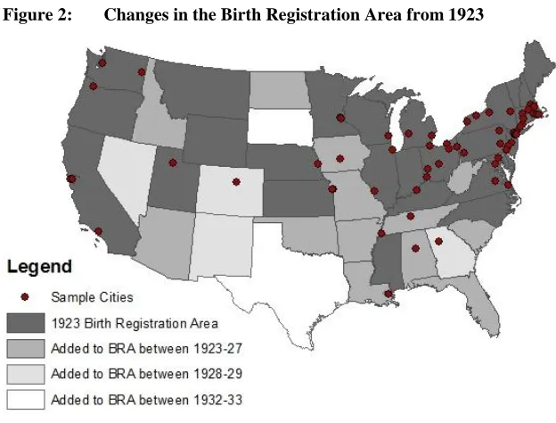
The BRAs consisted of about 60 percent of the U.S. in 1920, but grew throughout the decade so that by 1928, 44 states were officially recording births. Figure 2 maps the BRA states in 1923 and 1928, as well as the corresponding sample cities (cities over 100,000 persons in 1920 that had joined the BRA prior to 1928).

In the early 1920s, the Southeast and Central U.S were largely unrepresented in the BRA, yet by 1928 only New Mexico, Nevada, South Dakota, and Texas chose not to

5_{It is possible to construct TFR estimates at the municipal or county level by assuming that fertility schedules}

(14)

participate. Figure 3 plots the scaled GFR individually for four different BRA cities, as well as its average level in each year for all 64 sample cities.6 With the exception of a brief increase between 1923 and 1924, average fertility across the cities fell consistently between 1923 and 1932. The rates of decline, however, varied among cities. The four cities whose fertility levels are represented in Figure 3 are Fall River, MA, Camden, NJ, Los Angeles, CA, and San Francisco, CA, chosen for their differing fertility trajectories. Replacement level fertility is estimated to be approximately 2.3 during this period of time, and is indicated by the shaded area.7

Figure 2: Changes in the Birth Registration Area from 1923

Notes: BRA stands for “Birth Registration Area,” which consisted of the set of U.S. states recording birth information.

Camden, NJ and Fall River, MA started at similar position in the early 1920s, however by 1932 their fertility outcomes were very different. Aside from a slight increase in 1932, fertility in Fall River declined monotonically between 1923 and 1932,

6_{See the Appendix for a full list of each of the different cities included.}

7_{Replacement level is approximated by (1+SRB)/p(Am) where SRB is the sex ratio at birth. and p(Am) is the}

(15)

from almost 4 children per woman to below replacement level. The story differed in Camden, NJ, where fertility fluctuated above 3 children per woman with no clear trend over the study period. Fertility in Camden increased between 1923 and 1924, decreased in 1925 and 1926, and rose again in 1927 before falling through 1929, and then alternated between increasing and decreasing in 1930, 1931, and 1932. The second pair of cities in Figure 3 began the sample period at the bottom of the fertility distribution. While fertility in San Francisco decreased slowly throughout the 1920s and early 1930s, fertility in Los Angeles decreased rapidly. At the beginning of the decade, these cities were far apart in their fertility rates, but by the early 1930s, the gap had almost closed and both sat below a scaled GFR of 1.5. These were not the only cities that had reached such low fertility rates by the early 1930s. Portland, OR, and Kansas City, MO also had fertility rates below 1.5 during this year.

Figure 3: Total fertility rate trends

Notes: Fertility rates are the number of births per women aged 15 to 44 in each city, multiplied by 30 to make comparable to the TFR. Replacement level fertility is the level of fertility which would replace the population, accounting for sex ratios at birth and infant mortality.

Thus, some areas experienced much more rapid descents than others, even within the same geographic area. In some cases, the differences rivaled that of the often discussed urban/rural fertility difference. For example, in 1920 fertility in Fall River, MA was nearly 70 percent higher than fertility in San Francisco.

0 1 2 3 4

Sc

al

ed G

ener

al

F

ertility

Ra

te

Year

1933 Replacement level fertility: 2.3 San Francisco, CA

Los Angeles, CA

Average GFR Camden, NJ

(16)

These results show that the fertility decline varied across large U.S. cities during the 1920s. Many of the different explanations, outlined in Section 1, which have been shown to be important during other periods, are not entirely applicable to the period of the 1920s. Mean age at marriage was declining and urban economic outcomes were improving. For some U.S. urban areas, the Easterlin argument regarding the shift of the immigrant population may however be important. We propose and empirically test the claim that the programs to improve poor health and economic outcomes also played an important role in the 1920s fertility decline.

5. Data

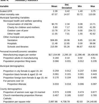
We estimate the relationship between public program investments and changes in fertility for a set of American municipalities with populations over 100,000 in 1920 and that were part of the BRA. The period under consideration is 1923–1932, chosen both for data availability reasons and to eliminate the effect of New Deal programs enacted after 1932. Information on the amount of spending distributed to these programs is obtained from the Financial Statistics of Cities volumes (U.S. Department of Commerce 1925–1936). These volumes also contain data regarding city expenditures on sanitation, health, and education. Per capita summary statistics adjusted to 2011 dollars for each of the spending variables are given in the top panel of Table 4. Population data by age and race were collected from the Decennial Censuses and interpolated for the inter-census years.

(17)

spending. Kansas City, KS and Scranton, PA, for example, waited until 1928 and 1930 to start investing in outdoor care of poor. Between 1923 and 1932, seven cities had periods of zero spending in this category.

Table 4: Summary statistics

Variable Mean Std.

Deviation Min Max

Scaled GFR 2.39 0.42 1.40 3.75

Infant mortality rate 67.07 14.07 33.72 110.00 Municipal Spending Variables Municipal health and welfare spending Conservation of child life $3.70 2.34 0.08 13.71 Charity for children and mothers 5.60 7.17 0.00 41.55 Outdoor care of poor 13.78 27.74 0.00 234.72 Other health 11.55 7.01 1.55 42.62 Other municipal cost payments Sanitation $36.89 18.06 8.85 111.66 Hospitals 11.48 12.65 0.00 99.96 Schools and libraries 215.99 55.26 86.87 416.92

Personal income/Economic variables

Manufacturing wages per worker $17,154.89 2,295.19 11,396.48 26,438.66 Proportion adults in manufacturing 0.184 0.10 0.02 0.51 Population proportion filing taxes 0.066 0.031 0.012 0.235

Municipal demographics

Proportion in city female & aged 1544 0.259 0.012 0.237 0.304 Proportion black female & aged 1544 0.081 0.101 0.001 0.443 Proportion foreign born female & age 1544 0.170 0.104 0.006 0.465

For persons over 10

Proportion illiterate 0.033 0.018 0.006 0.097

County demographics

Proportion of women over age 15 married 0.573 0.039 0.474 0.677

Church membership proportion Roman Catholic

0.457 0.185 0.037 0.765

Population per square mile 2,897.86 4,738.78 82.03 24,140.80

Notes: Government expenditures are per 100 persons and adjusted to 2011 dollars. Population figures are determined from the decennial censuses and interpolated.

(18)

Additional municipal spending data from the Financial Statistics of Cities volumes includes that for other health, sanitation, hospitals, and schools and libraries. Provision of public goods such as sanitation and schools and libraries may be correlated with the provision of other public goods, such as conservation of child life, and fertility. This is especially true with spending on education, because the department of education oversaw the medical inspections of school children in a few cities (U.S. Public Health Service 1923).

Other data, in addition to that collected from the Financial Statistics of Cities volumes, includes information on income and wealth in the different cities. Personal income information is unavailable at the city level prior to 1940, so we use average annual earnings from the manufacturing sector as a proxy. These are obtained from the Biannual Census of Manufactures volumes (U.S. Department of Commerce 1926– 1936).8 Using manufacturing wages in the different cities helps control for differences in economic conditions that may confound the relationship between investments in the different programs of interest and fertility. This may be especially important in the case of outdoor care of poor, as cities may have responded to poor economic conditions by increasing spending. The average manufacturing wages adjusted to 2011 dollars in Table 4 were about $17,200. To control for differences in the distribution of income, an additional measure of the number of tax returns filed in a year was collected from a series published by the U.S. Bureau of Internal Revenue (U.S. Bureau of Internal Revenue 1923–1932). This gives the number of jointly filing couples in each city with incomes above $5,000 and individual filers with incomes over $2,000 (respectively about $126,000 and $50,000 in 2011 dollars using contemporary standard of living values). Typically only about 6.5 percent of the population in the different cities filed taxes. The city with the highest proportion of filers was Los Angeles, with over a fifth of its population filing returns in 1923.

The demographics of a city are also possibly correlated with both public health and poverty relief spending, and fertility. The foreign born population generally had higher fertility than the native population, and also experienced worse health and economic outcomes (Duke 1915; Dempsey, 1919; Hughes 1923). In addition, since almost all births occurred within the institution of marriage, areas with higher proportions of married people would have higher levels of fertility. To control for changes in the population structure and other possible confounding demographic variables, municipal demographics for women of childbearing age were collected from the decennial censuses (U.S. Bureau of the Census 1921; 1931; 1942) and interpolated for the inter-census years. These include information on population density, the proportion over age

8

(19)

15 married, minority concentrations for women between the ages of 15 and 44, and literacy rates for individuals over the age of 10.

Church membership data is also included for the county-level proportion of individuals who belonged to the Roman Catholic Church. Moehling and Thomasson (2012) find that Roman Catholic Church membership negatively influenced state-level participation in the Sheppard-Towner Act, a federal public health education bill aimed at educating individuals in small cities and rural areas. If these policies also played out at the city level, and Roman Catholics have different fertility than other religious groups, then failure to control for the religious composition of a city will bias the coefficient estimates. In addition, the Roman Catholic Church was by far the largest church for the majority of this period, so this provides a good index for whether other religious groups were becoming a larger part of a city’s social structure. This ratio is calculated for each county by dividing the total number of church members in 1916, 1926, and 1936 by the number of Roman Catholic Church members and interpolating. This data is obtained from the 1916, 1926, and 1936 censuses of religious bodies (U.S. Bureau of the Census 1919; 1930; 1941).

6. Model and estimation

(20)

Table 5: Explaining spending with fertility

Dependent var: Conservation of child life spending

Outdoor care of poor spending

Charity for children and mothers

Prior year scaled GFR 0.0144 -0.259** -0.0165

0.009 (0.087) (0.016)

Constant -0.0090 0.7318** 0.0847+

(0.024) (0.236) (0.044)

City fixed effects Y Y Y

Year fixed effects Y Y Y

Observations 486 486 486

Within R-squared 0.358 0.542 0.238

Notes: Scaled GFR is a city’s General Fertility Rate, scaled to match the Total Fertility Rate scale.

Robust standard errors in parentheses. ** p<0.01, * p<0.05, + p<0.1. Government expenditures are per 100 persons and adjusted to 2011 dollars.

After controlling for spatial and temporal effects, prior year fertility is not significantly related to changes in spending for either conservation of child life or charity for children and mothers. Only for outdoor care of poor spending is the coefficient statistically different from zero. However, inclusion of the economic variables controlling for average annual manufacturing wages and the proportion of adults in manufacturing eliminates this statistical significance. Because variables are left out of the estimates presented in Table 5, these are not proof that changes in fertility in one year did not lead to changes in spending in the next. However, it is reassuring that after controlling for city and year fixed effects, a significant relationship does not remain. Although the existence of spending is likely associated with higher fertility levels in the different cities, year-to-year changes in spending are more plausibly exogenous. Thus, assuming that these unobserved factors that vary jointly with fertility and expenditures are not trending through time, it is possible to identify the relationship between these public programs and fertility using within city variation. Exploiting the panel structure of the data, we utilize this within variation through the use of a fixed effects model, defined below. Before presenting the model we discuss the appropriate lag structure.

(21)

appropriate for finding an effect. Thus we use a lag of two years.9 Any effect from the poverty relief programs on fertility is more likely to have an immediate effect. For these, a one year lag between expenditures and fertility is probably the most appropriate. We thus estimate the following model:

̂

∑

(1)

The dependent variable is the General Fertility Rate, ̂ , in city

i

and year

t

. The independent variable, , is the second lag of conservation of child life spending. The choice of only a second lag is based on considerations partly theoretical, as outlined above, and partly statistical. Statistically, the inclusion of the first lag of conservation of child life spending is neither economically not statistically significant, and does not affect the coefficient of the second lag. Theoretically, the educational nature of the conservation of child life programs meant that the activities engaged in under this spending likely took longer to percolate throughout a city than the welfare and poor relief payments of the other public programs studied here. Thus, for reasons of parsimony, we have included only the second lag of conservation of child life spending, and omitted the second lags of all other independent variables. For results from a model including the full distributed lag structure, please refer to the appendix.

1

,t

i

CCM

is per capita spending on charity for children and mothers in city

i

and

year

t



1

and is per capita spending on outdoor care of poor in city

i

and year

t



1

. To control for mortality influences on public program spending and

fertility, the lagged infant mortality rate,

IMR

_i_,_t_₁ is included. ∑ is a set of

J covariates that include the city demographic variables for the proportion of women between the age of 15 and 44, and the proportion of those women who were black or foreign born and between the ages of 15 and 44. The proportion of illiterate individuals over the age of 10, the proportion of women between the ages of 15 and 44 and married, the population density of the surrounding county, and the proportion of individuals in that county belonging to the Roman Catholic Church are included as well, as is the amount of prior year per capita spending on sanitation, hospitals, education, and health other than child health. In addition, X contains the income and income distribution measures and the proportion of adults working in manufacturing.

(22)

There may be still other factors influencing fertility. If these are jointly correlated with the spending variables of interest and fertility, then the model will not be identified. However, anything that is constant through time will be controlled for by the

set of city fixed effects, represented in the model by

C

_i. In addition, controlling for a

city-specific trend term, a state-specific trend term, or prior year fertility through an Arellano-Bond model does not significantly affect the coefficient estimates from equation (1). Estimates from these models are given in the appendix. Time-varying omitted variables can also confound estimates, so nationwide shocks common to all cities in the sample, due to changes in national optimism, shocks to national income, or

other factors, are controlled for with period effects

Y

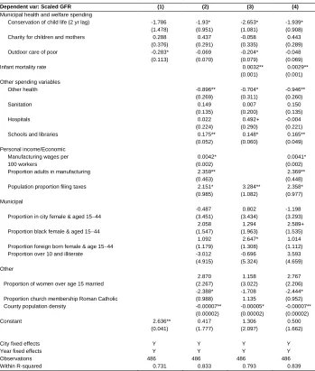
_t. Figure 3 suggests a common

(23)

Table 6: Fixed effects regression results

Dependent var: Scaled GFR (1) (2) (3) (4)

Municipal health and welfare spending

Conservation of child life (2 yr lag) -1.786 -1.93* -2.653* -1.939*

(1.478) (0.951) (1.081) (0.908)

Charity for children and mothers 0.288 0.437 -0.058 0.443

(0.376) (0.291) (0.335) (0.289)

Outdoor care of poor -0.283* -0.069 -0.204* -0.048

(0.113) (0.070) (0.079) (0.069)

Infant mortality rate 0.0032** 0.0029**

(0.001) (0.001)

Other spending variables

Other health -0.896** -0.704* -0.946**

(0.269) (0.311) (0.260)

Sanitation 0.149 0.007 0.150

(0.135) (0.200) (0.135)

Hospitals 0.022 0.492+ -0.004

(0.224) (0.290) (0.221)

Schools and libraries 0.175** 0.148* 0.165**

(0.052) (0.060) (0.049)

Personal income/Economic

Manufacturing wages per 0.0042* 0.0041*

100 workers (0.002) (0.002)

Proportion adults in manufacturing 2.359** 2.369**

(0.463) (0.448)

Population proportion filing taxes 2.151* 3.284** 2.358*

(0.985) (1.082) (0.977)

Municipal

Proportion in city female & aged 1544

-0.487 0.802 -1.198

(3.451) (3.434) (3.293)

Proportion black female & aged 1544

2.058 1.294 2.589+

(1.547) (1.963) (1.535)

Proportion foreign born female & age 1544

1.092 2.647* 1.014

(1.179) (1.308) (1.112)

Proportion over 10 and illiterate -3.012 -0.696 3.593

(4.915) (5.324) (4.659)

Other

Proportion of women over age 15 married

2.870 1.158 2.767

(2.267) (3.022) (2.206)

Proportion church membership Roman Catholic

-2.388* -1.708 -2.444*

(0.988) 1.135 (0.952)

County population density -0.00007** -0.00005* -0.00007**

(0.00002) (0.00002) (0.00002)

Constant 2.636** 0.417 1.306 0.500

(0.041) (1.777) (2.097) (1.662)

City fixed effects Y Y Y Y

Year fixed effects Y Y Y Y

Observations 486 486 486 486

Within R-squared 0.731 0.833 0.793 0.839

Notes: Robust standard errors in parentheses. ** p<0.01, * p<0.05, + p<0.1.

(24)

In the full model (4), of the key spending variables, only conservation of child life was significant statistically and economically, although spending on charity for children and mothers was also nearly statistically significant. In addition, alternative model specifications such as those in the appendix yield a positive and significant coefficient estimate for charity for children and mothers. Exclusion of the economic variables in Column 3 results in a coefficient estimate for charity and children and mothers close to zero. Because both average manufacturing wages and the proportion of workers in manufacturing are positively related to fertility, this suggests these variables are also negatively related to charity for children and mothers. Thus cities better off economically in a manufacturing sense spent less money on children in orphanages and mothers’ pensions. This gives some clue into the positive coefficient estimate, and suggests that an increase in the number of poorer individuals led to both increases in municipal spending on almshouses and mothers’ pensions as well as fertility. For outdoor care of poor, the opposite is true: its estimated coefficient is significant only with the exclusion of the economic variables. Thus outside of being a proxy for changing economic circumstances, spending on outdoor care of poor does not seem to be important in explaining fertility changes in the 1920s. Conversely, the coefficient on conservation of child life is significant in most versions of equation 1. Exclusion of the infant mortality rate only marginally affects the coefficient on conservation of child life spending, suggesting that the child health programs were not related to fertility through their effects on infant mortality.

Other variables with statistically significant coefficients include infant mortality, spending on other health, spending on schools and libraries, manufacturing wages, the proportion of adults in manufacturing, the proportion of the population that filed taxes, the proportion of the population female aged 15 to 44 and black, the proportion of church membership which was Roman Catholic, and the county population density. Although each of these relationships is interesting in their own light, their importance in the context of this paper is of secondary nature.

(25)

the Children’s Bureau that African-American families had higher levels of fertility than native white families, which may explain the positive relationship between fertility and this demographic variable.

The negative relationships identified for the independent variables included spending on other health, the proportion of church membership which was Roman Catholic, and the population density of the surrounding county. Spending on “other health” was a combination of expenditures on health administration, vital statistics, prevention and treatment of diseases, and the regulation of food and dairy; and so increases in municipal health investments seem to have been followed by reductions in fertility. The same was true for the proportion of church membership which was Roman Catholic. The negative coefficient estimated by the model is most likely a result of the growing influence of the Baptist churches during this time. For areas that experienced changes in their religious compositions, this was often due to increases in the Baptist population at the expense of the Roman Catholics. The higher fertility of the Baptist followers would then explain this negative relationship. Lastly, cities located in more densely populated counties tended to have lower levels of fertility.

With regard to magnitudes, none of the coefficient estimates suggest that a single factor was the primary driver of the decline. The coefficient on IMR is economically significant, yet it explains only a small portion of the fertility decline. Across all cities, IMR declined from an average of 78.5 deaths per thousand live births in 1923 to 55.9 deaths per thousand live births in 1932. The average annual decline of IMR then being about 2.25, the estimated coefficient of 0.0029 implies a 0.0065 reduction in the overall General Fertility Rate (about -0.24% from the 1923 average GFR of 2.74).

Comparing the magnitudes of the coefficients to each other, manufacturing wages would on average need to increase by 75 percent to create a 0.5 increase in the average GFR. Conversely, a 20 percent change in the proportion of people filing would generate about the same effect. Of the demographic variables, a 0.1 unit change in the proportion of individuals female, African American, and between the ages of 15 and 44, would tend to increase fertility by about 0.2 points. For education, a $60 increase in spending is associated with a 0.1 increase in GFR. The largest annual change in education spending for any city in the sample between 1923 and 1932 was about $90, so this level is fairly high relative to what cities were spending.

(26)

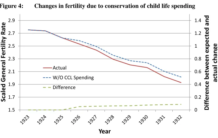
estimate indicates about the role of the conservation of child life expenditures for the 1920s fertility decline. Based on these estimates, Figure 4 constructs what fertility rates would have looked like if cities held all other forms of spending constant, but eliminated conservation of child life expenditures. Although this is an extrapolation from reality, it is helps illustrate the sense of relative importance of the conservation of child life spending. The predicted trend without conservation of child life spending plotted in Figure 4 is constructed by calculating the actual annual change, and then subtracting the estimated effect from spending in year . This works out to:

̂ (2)

Figure 4: Changes in fertility due to conservation of child life spending

Notes: CCL stands for “Conservation of Child Life”.

The predicted trend without CCL spending plotted is constructed by calculating the actual change in each year, then subtracting the estimated effect (Table 6, Column 4) from spending in year .

0 0.2 0.4 0.6 0.8 1 1.2 1.4 1.5 1.7 1.9 2.1 2.3 2.5 2.7 2.9

Diff

er

enc

e

be

tw

een

exp

ect

ed

and

actual

chang

e

Sca

led

Gen

er

al F

ertility

Ra

te

Year

Actual

W/O CCL Spending

(27)

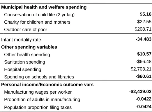
Table 7: Change necessary for 0.1 decrease in fertility

Municipal health and welfare spending

Conservation of child life (2 yr lag) $5.16 Charity for children and mothers $22.55 Outdoor care of poor $208.71

Infant mortality rate -34.483 Other spending variables

Other health spending $10.57 Sanitation spending -$66.48 Hospital spending $2,703.21 Spending on schools and libraries -$60.61 Personal income/Economic outcome vars

Manufacturing wages per worker -$2,439.02 Proportion of adults in manufacturing -0.0422 Population proportion filing taxes -0.0424

Notes: Estimates are based off of the coefficients given in Table 6, Column 4. Unless otherwise noted, the relationships are between TFR hat and the 1 year lag of the different variables. Bolded values indicate a statistically significant relationship at the 0.1 level.

The estimate in Table 6 suggests that, if municipalities during the 1920s and early 1930s did not invest in the conservation of child life programs, fertility rates would have been about 5 percent higher. Alternatively, the conservation of child life programs explain about 10 percent of the change in fertility in 1920–1932. Variations in spending across areas also explain some of the city level variation. For cities in a state such as New Jersey, which invested heavily in the conservation of child life programs, the coefficient estimates potentially explain as much as 20 to 40 percent of the fertility decline for the different cities. Many of the cities in Ohio, on the other hand, invested less in these programs. For these areas, the coefficient estimates potentially explain only around 7 percent of the fertility decline that occurred.

(28)

their contribution to health, or perhaps through their advocacy of practices such as breast feeding, birth spacing, and smaller families, tended to experience more rapid declines in fertility.

7. Conclusion

Aside from the baby boom of the 1940s and 50s and the slow fertility increase starting in the 1970s,10 fertility in the U.S. has been declining since the mid-1800s. A variety of reasons for this overall negative trend have been offered, likely because different reasons have proven to be important during different periods. During the 18th Century, it was likely the increasing price of land and associated increase in the age of marriage (Hacker 2003). Increases in per capita income, and the opportunity costs and substitution effects that come with those increases, have also been shown important (Jones and Tertilt 2008). Fertility control has certainly played a role, as well as the numerous demographic shifts which have occurred over the history of the U.S. To these different explanations, we would like to offer support for the contributing factor of public policy decisions. We do not know if reducing fertility was a subtle, unstated goal of the conservation of child life programs administered in the different municipalities, but the presence of these programs were significantly related to the fertility declines that these areas experienced.

Some of the cities analyzed invested relatively heavily in these programs, while others invested relatively light in the years 1923–1932. Fertility patterns also varied strongly across areas on the same period, and this variation in fertility has continued to be the case in the U.S. These differences across areas are due to a multitude of cultural and economic factors, outside the scope of this study. For a fuller understanding of regional differences in fertility across the U.S., please see Lesthaeghe and Neidert (2006). We would like to point out, however, that differences in investment in certain types of public programs, specifically conservation of child life, potentially offer one additional reason for why different cities experienced different fertility outcomes in the 1920s and early 1930s. Although these programs were instituted as a means for reducing mortality and did not explicitly target fertility, it appears this was one of their effects.

10

(29)

8. Acknowledgements

(30)

References

Andreev, E.M. and Shkolnikov, V.M. (2012). An Excel spreadsheet for the decomposition of a difference between two values of an aggregate demographic measure by stepwise replacement running from young to old ages. Rostock: Max Planck Institute for Demographic Research (MPIDR Technical Report TR– 2012–002).

Andreev, E.M., Shkolnikov, V.M., and Begun, A.Z. (2002). Algorithm for decomposition of differences between aggregate demographic measures and its application to life expectancies, healthy life expectancies, parity–progression ratios and total fertility rates. Demographic Research 7(14): 499–522.

doi:10.4054/DemRes.2002.7.14.

Barro, R.J. and Becker, G.S. (1989). Fertility Choice in a Model of Economic Growth.

Econometrica 57(2): 481–501. doi:10.2307/1912563.

Becker, G.S. (1960). An economic analysis of fertility. In: National Bureau of Economic Research (ed.). Demographic and Economic Change in Developed Countries. Princeton: Princeton University Press: 209–240.

Becker, G.S. and Tomes, N. (1976). Child endowments and the quantity and quality of children. Journal of Political Economy 84(3): 143–162. doi:10.3386/w0123.

Bongaarts, J. (1978). A Framework for Analyzing the Proximate Determinants of Fertility. Population and Development Review 4(1): 105–132. doi:10.2307/ 1972149.

Bongaarts, J. (1987). The proximate determinants of fertility. Technology in Society 9(3–4): 243–260. doi:10.1016/0160-791X(87)90003-0.

David, P.A. and Sanderson, W.C. (1987). The Emergence of a Two–Child Norm among American Birth–Controllers. Population and Development Review 13(1): 1–41.

doi:10.2307/1972119.

Dempsey, M.V. (1919). Infant mortality: Results of a field study in Brockton, MA based on births in one year. Washington D.C.: Government Printing Office.

Doepke, M. (2005). Child mortality and fertility decline: Does the Barro-Becker model fit the facts? Journal of Population Economics 18(2): 337–366. doi:10.1007/ s00148-004-0208-z.

(31)

Easterlin, R.A. (1961). The American baby boom in historical perspective. The American Economic Review 51(5): 869–911.

Eckstein, Z., Mira, P., and Wolpin, K.I. (1999). A Quantitative Analysis of Swedish Fertility Dynamics: 1751–1990. Review of Economic Dynamics 2(1): 137–165.

doi:10.1006/redy.1998.0041.

Fishback, P.V., Haines, M.R., and Kantor, S. (2007). Births, Deaths, and New Deal Relief during the Great Depression. Review of Economics and Statistics 89(1): 1–14. doi:10.1162/rest.89.1.1.

Guinnane, T.W. (2011). The Historical Fertility Transition: A Guide for Economists.

Journal of Economic Literature 49(3): 589–614. doi:10.1257/jel.49.3.589.

Hacker, J.D. (2003). Rethinking the “early” decline of marital fertility in the united states. Demography 40(4): 605–620. doi:10.1353/dem.2003.0035.

Haines, M.R. (2000). The white population of the United States, 1790–1920. In: Haines, M.R. and Steckel, R.H. (eds.). A Population History of North America. New York: Cambridge University Press: 305–370.

Haines, M.R. and Guest, A.M. (2008). Fertility in New York state in the pre–civil war era. Demography 45(2): 345–361. doi:10.1353/dem.0.0009.

Hirschman, C. (1994). Why Fertility Changes. Annual Review of Sociology 20(1): 203– 233. doi:10.1146/annurev.so.20.080194.001223.

Hughes, E. (1923). Infant mortality: Results of field study in Gary, Ind., based on births in one year. Washington D.C.: Government Printing Office.

John, A.M., Menken, J.A., and Chowdhury, A.K.M.A. (1987). The Effects of Breastfeeding and Nutrition on Fecundability in Rural Bangladesh: A Hazards– Model Analysis. Population Studies 41(3): 433–446. doi:10.1080/

0032472031000142986.

Jones, L.E. and Tertilt, M. (2008). An economic history of fertility in the U.S.: 1826– 1960. In: Rupert, P. (ed.). Frontiers of Family Economics. Emerald Group Pub.: 165–230.

Lancaster, L.W. (1937). Government in rural America. New York: D. Van Nostrand Company.

(32)

Lathrop, J.C. (1919). Income and infant mortality. American Journal of Public Health 9(4): 270–274. doi:10.2105/AJPH.9.4.270.

Lesthaeghe, R.J. and Neidert, L. (2006). The Second Demographic Transition in the United States: Exception or Textbook Example? Population and Development

Review 32(4): 669–698. doi:10.1111/j.1728-4457.2006.00146.x.

Meckel, R.A. (1990). Save the Babies: American Public Health Reform and the Prevention of Infant Mortality, 1850–1929. Ann Arbor: University of Michigan Press.

Moehling, C.M. and Thomasson, M.A. (2012). The Political Economy of Saving Mothers and Babies: The Politics of State Participation in the Sheppard-Towner Program. The Journal of Economic History 72(1): 75–103. doi:10.1017/S002205 0711002440.

Myrskylä, M., Kohler, H.–P., and Billari, F.C. (2009). Advances in development reverse fertility declines. Nature 460(7256): 741–743. doi:10.1038/nature08230.

Newmayer, S.W. (1911). The Warfare Against Infant Mortality. The ANNALS of the

American Academy of Political and Social Science 37(2): 288–298. doi:10.1177/

000271621103700224.

Sah, R.K. (1991). The Effects of Child Mortality Changes on Fertility Choice and Parental Welfare. Journal of Political Economy 99(3): 582–606. doi:10.1086/ 261768.

Sanger, M. (1931). The pro and con feature: Proposed federal legislation on birth control. Congressional Digest 10(4): 104–108.

Skocpol, T., Abend–Wein, M., Howard, C., and Lehmann, S.G. (1993). Women's Associations and the Enactment of Mothers' Pensions in the United States. The

American Political Science Review 87(3): 686–701. doi:10.2307/2938744.

Smith, M.P. (1932). Trends in Municipal Administration of Public Welfare: 1900– 1930. Social Forces 10(3): 371–377. doi:10.2307/2569677.

Sobotka, T., Skirbekk, V., and Philipov, D. (2011). Economic Recession and Fertility in the Developed World. Population and Development Review 37(2): 267–306.

doi:10.1111/j.1728-4457.2011.00411.x.

(33)

U.S. Bureau of Internal Revenue (1923–19362). Statistics of Income. Washington, D.C.: Government Printing Office.

U.S. Bureau of the Census (1919). Religious bodies: 1916. Washington, D.C.: Government Printing Office.

U.S. Bureau of the Census (1921). Fourteenth census of the United States taken in the year 1920. Washington, D.C.: Government Printing Office.

U.S. Bureau of the Census (1931). Fifteenth census of the United States taken in the year 1930. Washington, D.C.: Government Printing Office.

U.S. Bureau of the Census (1942). Sixteenth census of the United States: 1940. Washington, D.C.: Government Printing Office.

U.S. Bureau of the Census (1975). Historical statistics of the United States, colonial times to 1970, bicentennial edition. Washington, D.C.: Government Printing Office.

U.S. Bureau of the Census (2011). Statistical abstract of the United States: 2012 (131st edition). Washington, D.C.: Government Printing Office.

U.S. Children’s Bureau (1919). Our Children. Film.

U.S. Department of Commerce (1922–1923). Birth statistics for the birth registration area of the United States. Washington, D.C.: Government Printing Office.

U.S. Department of Commerce (1924–1934). Birth, stillbirth and infant mortality statistics. Washington, D.C.: Government Printing Office.

U.S. Department of Commerce (1925–1936). Financial statistics of cities. Washington, D.C.: Government Printing Office.

U.S. Department of Commerce (1926–1936). Biennial census of manufactures. Washington, D.C.: Government Printing Office.

(34)

Williamson, S.H. (2015). Seven ways to compute the relative value of a U.S. dollar

amount, 1774 to present [electronic resource]. MeasuringWorth.

http://www.measuringworth.com/uscompare/

(35)

Appendices

A. Alternative measures of municipal fertility rates

The primary text measures municipal fertility using a scaled version of the General Fertility Rate. This is the simple ratio of the total number of births to the number of women between the ages of 15 and 44, multiplied by 30. Normally this ratio is multiplied by 1000; however, we wished it to be on the same scale as the Total Fertility Rate (TFR). When the data allows, use of this TFR is preferable, as it allows for controlling of the age structure of fertility. which may vary across areas.

Although births by age are not available at the city level during the sample period, it is possible to construct municipal TFRs using the age structure of the state or the overall Birth Registration Area (BRA) in which each city resides. We name the TFR that uses the age structure of the state in which each city resides the , and the TFR that uses the age structure of the overall Birth Registration Area the ̂. We begin with the description of the latter.

In order to calculate ̂ for each city in the sample, we estimate the municipal age specific birth rates using the BRA as a whole. The age-specific birth rates are defined as BRAt

x

nF

, _{, where}

_n

_{is the length of the age group (5 years),}

_x

_{is the age}

group (15 to 19, 20 to 24, 25 to 29, 30 to 34, 35 to 39, or 40 to 44),

BRA

indicates that this is for the entire Birth Registration Area, and

t

is the time period reference. Because of the expansion of the BRA between 1920 and 1933, different years will see different sets of participating states. See Table C1 for an accounting of BRA entry for each of the different states. We express the age specific birth rate for those areas participating in the BRA as:

(A1)

t BRA x n

B

,

is the number of births in a specific age group and _n

P

_xBRA,t is the female

population within that age group. These age specific fertility rates are then used to

create a proportion _n



BRA_x , where

(36)

Here, α is the minimum age at childbearing, which we set at 15, and β is the maximum age at childbearing, which we set at 44. The age-specific births for each city i are then:

̂

(A3)

t i

R

F

T

ˆ

, is then:

̂

_∑

̂

(A4)

The second calculation of the municipal TFRs uses a finer level of detail. For , the state-level age-specific fertility rates are used in place of rates from the entire BRA. Thus, the age-specific birth counts _n

B

ˆ

_xi,t are calculated using a



calculated at

the state level. Specifically,_n

B

ˆ

_xi,t



_n

B

i,t

*

_n



s_x,t, where s is the state in which city i lies.

The age-specific birth counts are then used to estimate . Estimates from the models substituting and ̂ for the scaled General Fertility Rate as presented in Section 6 are given in Table A1.

(37)

Table A1: New dependent variables results

Dependent var: TFR hat TFR*

Municipal health and welfare spending Conservation of child life (2 yr lag) -1.977* -1.961*

(0.889) (0.899)

Charity for children and mothers 0.445 0.457

(0.278) (0.281)

Outdoor care of poor -0.041 -0.042

(0.064) (0.064)

Infant mortality rate 0.0028** 0.0028**

(0.001) (0.001)

Other spending variables