Optimization-based non-linear Control Law with Increased Robustness for Air Fuel Ratio Control in SI Engines

(1)

Robustness for Air Fuel Ratio Control in SI Engines

A.Amini, M. Mirzaei, R. Khoshbakhti Saray

Faculty of Mechanical Engineering, Sahand University of Technology, Tabriz, Iran.

Abstract

In spark ignition (SI) engines, the accurate control of air fuel ratio (AFR) in the stoichiometric value is required to reduce emission and fuel consumption. The wide operating range, the inherent nonlinearities and the modeling uncertainties of the engine system are the main difficulties arising in the design of AFR controller. In this paper, an optimization-based nonlinear control law is analytically developed for the injected fuel mass flow using the prediction of air fuel ratio response from a mean value engine model. The controller accuracy is more increased without chattering by appending the integral feedback technique to the design method. The simulation studies are carried out by applying severe changes in the throttle body angle to evaluate the performance of the proposed controller with and without integral feedback. The results show that the proposed controller is more effective than the conventional sliding mode controller in regulating the AFR without chattering.

Keywords: SI engine; Air fuel ratio; Non-linear control; Optimization; Increased robustness

1. Introduction

Nowadays, the control of internal combustion (IC) engines becomes an important topic for automobile engine researchers. This is for the reason that the car manufacturers strongly need to reduce the fuel consumption and emission below the standards while maintaining the best performance for the engine. In order to meet the mentioned requirements, different engine variables need to be controlled. Among them, controlling the air fuel ratio (AFR) in the stoichiometric value can mostly influence on emissions and performance characteristics of the engine [1-3].

Regularly, the products of incomplete combustion of IC engines are reduced by three way catalyst (TWC). This convertor is mounted in the exhaust pipe and can oxidize NOx, CO and HC, simultaneously. The maximum efficiency of TWC is achieved when the AFR is close to the stoichiometric value. In most cases, the relative proportion of air and fuel ratio can be stated in terms of the lambda ratio () which is defined as the actual AFR divided by the stoichiometric AFR. For the lean mixture combustion in which the AFR is greater than the stoichiometric value ( > 1), the amounts of CO and HC are increased, while for the rich mixture combustion ( < 1), more NOx is produced [4]. To avoid these

two undesired conditions, the lambda ratio should be maintained close to one ( = 1), especially in the transient range of engine operation. This aim is realized by the control of injected fuel mass flow that is applied with injectors.

In order to design a suitable AFR control law applicable to a wide range of engine operations, the nonlinear air induction and fueling dynamics should be employed in the design model. Moskwa [5] performed extensive works in this field and conducted series of experiments in General Motors research laboratories. As a result, a real time control model was developed and accordingly nonlinear algorithms were invented for automotive engine control. Hendricks and Sorenson [6] proposed the mean value engine model (MVEM) that is suitable for applying model-based control methods.

In the development of AFR controllers, the sliding mode control (SMC) methods have been frequently applied because of their potential to cope with nonlinearities and intrinsic robustness. Kaidantzis et al. [7] used the sliding mode method for the air fuel ratio control, but the designed controller was not efficient for rapid changes of the throttle body. Souder and Hedrick [8] employed adaptive sliding mode method to determine the sliding gain. Their controller was applicable for extensive engine operating conditions especially when sensor delays

(2)

are included in the model. However, one of the undesirable effects of the sliding mode control in practice is the chattering phenomenon which is caused by the system uncertainties and the time delay in crankshaft, fuelling and oxygen sensor dynamics. In order to reduce the chattering, Wang and Yu [1] developed the second order sliding mode method for the AFR control and achieved the improved control performance compared with the conventional SMC. In this work, the derivative of control input was derived from the control law and therefore the actual control input, the injected fuel mass flow, was obtained by the integration method. The other important control methods used for the AFR control are the following: linear parameter- varying control [2], proportional-integral-derivative (PID) control [3], neural networks [4] and fuzzy-based techniques [9].

Recently, authors developed an optimization-based nonlinear control law for control of AFR optimization-based on the generic mean value engine model [10]. The Lambda sensor dynamics is also employed in the design model. The proposed control law is developed by minimizing the difference between the AFR response predicted from the nonlinear engine model with four states and the stoichiometric AFR as the desired value. The similar predictive control approach has been already developed by the research team of authors for control of vehicle yaw dynamics [11] and anti-lock braking system [12].

In the present study, to improve the AFR controller performance designed in [10], the integral feedback technique is appended to the proposed control method in order to increase the robustness of the designed controller in the presence of model uncertainties without chattering. In fact, the accurate control of air fuel ratio in the presence of model uncertainties is achieved by minimizing both the AFR error and its integral. The capability of the different versions of the designed controller, with and without integral feedback, in maintaining the stoichiometric value of AFR is investigated by applying severe changes in the throttle body angle. At the end, the performance of the proposed controller is compared with that of a conventional sliding mode controller in the presence of modeling uncertainties.

2. Engine model

The engine model described here is based on the generic mean value engine model [13-14]. This model has four subsystems including intake manifold dynamics, crankshaft dynamics, fuel injection dynamics and oxygen sensor dynamics. The injection mass flow is the control input and the throttle body angle is considered as the disturbance input of the

system. In the following, the goverining equations of each subsystem are described. All variables of the model are defined in the notation.

2.1 Intake manifold filling dynamics

In this study, the intake manifold is modeled based on the isothermal assumption. By considering the validity of the ideal gas law and that the intake manifold temperature is accurately known, the equation of the manifold pressure in terms of the air mass flow past the throttle plate and the air mass flow into the intake port is described as

The air mass flow past the throttle plate (

m

&

at_{) is} related to the throttle position and the manifold pressure:

Where

= 1 − cos −

2 3 =

4

, , and are constants.

Also, the air mass flow into the intake port () is determined by the Speed-density equation as follows:

where

and were calculated for different engines in [13].

2.2 Crankshaft dynamics

The equation of engine speed is derived by using the conservation of rotational energy on the crank shaft as follows [14]:

p!=RT_V!

! %m'(− m')* 1

, =

,-

+ 2

= /01 − 1

−

1 − 2

1 34 <

34 ≥ 5

7, = 78_120;-9

<= 6

<== + 7

7 = −_{@. 7 BC}1 D, 7 + C, 7 + CE7F

+_{@. 7 G}1 H<, 7DI

− ΔK9 8

(3)

where the crankshaft load inertia @ is

The friction power (C_D) and the pumping power (C) are functions of the intake manifold pressure and the engine speed, which can be described by the following equations:

There are many difficulties in determination of the engine load (C_E) which is required to solve the engine speed equation (8). For simplicity, it is assumed that the engine load is a function of the engine speed as follows [6]:

The thermal efficiency (

η

i_{) is written as a product}

of two terms:

For the engine examined in its operating range, the following functions can be written [9]:

Since the injected fuel has a delay to produce the corresponding power, the following injection-power stroke delay is described:

where n is in RPM.

2.3 Fuel injection dynamics

The fuel film dynamics in a SI automotive engine can be described as follows:

where

and _DD is obtained by integration of the following equation

The time constant K_D for the fuel evaporation together with the fuel proportion M_D that is deposited on the intake manifold wall or close to the intake valves are dependent on the operating point and vary for different engines. An example of the mentioned

parameters for a specific engine in terms of the model states is given as follows [14]:

Note that the fuel flow rate is bounded between 0 and 0.004 kg/s. This restriction is important when simulating the performance of the controller because it is unrealistic to allow the controller to command negative or infinite fuel [8].

2.4 Sensor dynamics

The oxygen sensor or the air fuel ratio sensor is used for determination of oxygen concentration in exhaust gas contents. The dynamic behavior of sensor response is modeled as a transport delay followed by a first lag [15]:

where _N is the lambda ratio that is measured by the sensor and is the lambda ratio of induced mixture:

The engine cycle delay is described as:

where n is in RPM.

The unavoidable time delay between and _N causes the uncertainty in the problem.

3. Control System Design

3.1 Development of the control law

The nonlinear engine system dynamics described in section 2 can be written in the state space form by considering _N as the output of the system

Where X is the state vector and u is the control input

The first and second state equations are directly written from equations (1), (8). The third equation can be written from equations (17) - (19) as follows

@ = @B_30FO

× 1000 9

CD, 7 = 71.673 + 0.2727 + 0.01357 10

C, 7 = 7−0.969 + 0.2067 11

CE7 = RE7S 12

<, 7 = <<T7 13

< = 0.9301 + 0.215− 0.1657 14

<T7 = 0.5581 − 0.3927U.SV 15

ΔK9=60_{7 W1 +}₇1 XYZ 16

D= D=+ DD 17

D== %1 − MD*D 18

[DD=_K1 D%−DD+ MDD* 19

KD= 1.351.68 − 0.6727− 0.825 + 0.15 − 0.067 + 0.56 20

MD= −0.277− 0.0557 + 0.68 21

K\NI + NI = I − ] 22

= D^_;` 23

] = 1a_{720 2 W}bcd ₇120 XY. 7Z + I9 24

eM = 4M, f_{g = h} i 25

M = j h h hS hi k = j 7 D N k 26

f = D 27

(4)

At the end, by substituting equations (23) in (22), the fourth state equation can be written as:

Now, according to the above state equations, an optimization-based non-linear control law is developed for the design of AFR controller. Briefly, the non-linear response of lambda for the next time interval, I + ℎ, is first predicted by Taylor series expansion and then the current control fI will be found based on continuous minimization of predicted tracking error. The predicted period h is a real positive number. In order to further increase the robustness of the lambda controller, the integral of lambda is appended to the state equations. In this technique called integral feedback [16], the new state variable x5 is defined as follows:

hm= hi 30

The purpose of control system is to maintain the lambda, h_i= and its integral, h_m= n oI, close to their desired responses. These two state variables are considered as the outputs of the system, g =

phi, hmqr . Therefore, a pointwise minimization performance index that penalizes the tracking errors at the next instant, yet is not excessive, is considered in the following form:

This can be written as :

Note that, to achieve the perfect tracking, the weighting term of the control input fI is not included in the performance index. This case is considered as the cheap control [7, 8].

First approximate each h_TI + ℎ by a R_Tth-order Taylor series at

Note that, to achieve the perfect tracking, the weighting term of the control input fI is not included in the performance index. This case is considered as the cheap control [7, 8].

First approximate each h_TI + ℎ by a R_Tth-order Taylor series at:

Now, the key issue is to choose the order R_T for each output in a way that is suitable for the purpose of controller design on the basis of predictions. The expansion order, which specifies the highest order derivative of each output used in the prediction, is determined by the relative degree of the nonlinear system [11-12, 17].

According to the equations (29) and (30), the system dynamics has the well-defined degrees,

si= 1 and s_m= 2 relative to the outputs g= h_i and g= h_m, respectively, which are determined as the lowest order of the derivative of each output in which the input u first appears explicitly [18]. Therefore, the first order Taylor series is sufficient for the expansion of h_i, but at least the second order Taylor series is required for the expansion of h_m

Substituting Eqs. (29) and (30) into (34) and (35) yields

In the above equation, the relation h[_m= h_i is used from equation (30). Also, the desired states can be expanded in the same manner as before

Now, the expanded performance index can be obtained as a function of control input by substituting equations (36) - (39) into (32)

The necessary condition for optimality is

This leads to

hS= 1 − MDf +_K1

\1−DD+ MDtfoI2 28

hi=_K \^_;`hS−

hi

K\ 29

u =1_{2 v}iphiI + ℎ − hi9I + ℎq

+1_{2 v}mphmI + ℎ

− hm9I + ℎq 31

u =1_{2 w v}TphTI + ℎ − hT9I + ℎq 32 m

Txi

hTI + ℎ = hTI + ℎhTI +y

z

!h[TI + ⋯ + y}~

~!hT

~_{I 7 = 4,5}₍₃₃₎

hiI + ℎ = hiI + ℎhi 34

hmI + ℎ = hmI + ℎhmI +ℎ

2 h[mI 35

hiI + ℎ = hiI + ℎ 1_K \^_;`hS−

hi

K\2 36

hmI + ℎ = hmI + ℎhiI

+ℎ_{2 1} _K

\^_;`hS−

hi

K\2 37

hi9I + ℎ = hi9I + ℎhi9I 38

hm9I + ℎ =

hm9I + ℎhi9I +y

z

hi9I 39

u =vihiB1 −yF +yN− hi9

+vmhm+ hiℎ B1 −yF + y

z_N

− hm9− ℎhi9

40

u

f = 0 41

(5)

Where _i and _m are the current tracking errors

and is the weighting ratio

=v_vm

i 45 Equation (42) describes a nonlinear lambda control law containing the integral feedback. The special case of the control law considering no integral feedback can be easily derived by taking the weighting factor of the integral state, h_m, to be zero in the performance index (31), i.e. v_m= 0. In this case, the weighting ratio will be zero from equation (45). Therefore, the lambda control law without integral feedback is achieved as follows:

By applying the control law (46), described without integral feedback, in the engine model (29), the error dynamics of lambda in the closed loop system is obtained as follows:

Clearly, the error dynamics (47) is linear and time invariant. It is seen that this version of control law naturally leads to a special case of input/output linearization. In this way, the closed-loop system is linear and exponentially stable for anyℎ > 0 . According to error dynamics, as the initial error is zero, the perfect regulation of lambda is maintained for all time in the absence of model uncertainties.

Also, it is considered from the error dynamics (47), the prediction time ℎ plays the role of time constant of the closed loop system. Therefore, the transient error can be decreased through small values of ℎ. As a result, when the modeling uncertainties exist in the system, the arisen transient and steady state errors can be decreased by the regulation of the free parameter ℎ. However, in order to decrease the error in the presence of persistent uncertainties, the value of ℎ can be decreased to some extend, otherwise the chattering problem will be appeared and the control energy will be oscillatory [12]

.

Table1. Engine specifications

Properties symbol Value(unit)

Engine displacement Vd 1.275 liter

Manifold volume Vi 1.692e-3 m3

Number of cylinders ncyl 4

Engine load inertia Iac 0.48 kg.m2

Fuel lower heating value Hu 43000 kJ/kg

Intake manifold temp Ti 293 K

Idle speed throttle angle α₀ _{15 degree}

Sensor lag time constant τ_d _{85 ms}

Exhaust valve open θ

EVO 500 degree

Exhaust transport delay td 4.2 ms

%1 − MD*f + 1−_KDD

\ +

MD K\tfoI2

=

−ℎ

K\^_;`11 + ℎ 4 2 hiB1 − ℎK_\F − hi9+ ℎ2 1m+ ℎi− ℎ

2K\hi2

42

i= hiI − hi9I 43

m= hmI − hm9I 44

%1 − MD*f + 1−_KDD

\ +

MD K\tfoI2

= −ℎ

K\^_;`

hiB1 − ℎK_\F − hi9

46

i+1_ℎi= 0 47

(6)

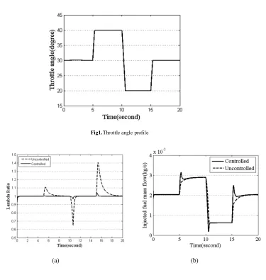
Fig1.Throttle angle profile

(a) (b)

Fig2.Simulation results of AFR for the system with and without control (a) Injected fuel mass flow (b) Lambda ratio

To overcome this problem and to eliminate the steady state regulation error without any oscillation in the control energy, the control law (42) with integral feedback should be used in the engine system. In this way, by selecting a suitable value for the weighting ratio , the transient error arisen from the persistent uncertainty is remarkably decreased and the steady state regulation error is also eliminated. This fact is more clarified by the simulation studies in which the error dynamics of different controllers are numerically solved and compared.

3. Simulation Results

Simulation studies are conducted using a four-cylinder spark ignition engine model to evaluate the

performance of the proposed controller with different versions. The model specifications are shown in Table 1. To simulate different operating conditions, the throttle angle is designed to change from 20 degree to 40 degree in rising time of 0.3 second and falling time of 0.6 second as shown in Figure 1. In this condition, the engine speed is varied between 2200 rpm and 4200 rpm.

In order to emphasize the necessity of controlling the AFR in the engine system, the responses of the uncontrolled engine is compared with that of the controlled one. For the uncontrolled engine, the wall wetting is neglected and the injected fuel mass flow is calculated by _D= /^_;_`.

Figure 2a compares the injected fuel mass flow of the engine in controlled and uncontrolled cases. Accordingly, the calculated lambda ratios for both

(7)

cases are compared in Fig. 2b. As it is considered, the designed controller can successfully keep the AFR near the stoichiometric value even for the rapid changes of throttle angle at 5th, 10th and 15th seconds. In contrast, for the engine without the controller, the air fuel ratio has intensive fluctuations when a rapid change of throttle angle is applied. This is for the reason that when the throttle is opened rapidly, the air flow is greater than the fuel flow and consequently the lambda ratio is greater than one. It means that the air fuel mixture is lean. This excursion is occurred because the intake manifold filling dynamics is faster than the fuel injection dynamics. Also, when the throttle is closed rapidly, the AFR has a tendency to be rich.

In the simulation study considered above, no modeling uncertainty is supposed. Therefore, the control law without integral feedback is suitable for the control system. In order to evaluate the robustness of the designed controller in the presence of modeling parametric uncertainties, the previous

changes in the throttle angle are considered again. It is assumed that the uncertainties have risen out of 10% uncertainty in port air mass flow and 10% uncertainty in lambda sensor signal. First, the control law (46), without integral feedback, is employed. The effect of the structured uncertainty in engine parameters is evaluated in Figure 3a for different values of prediction time h. The result indicates that the modeling uncertainty as a disturbance input causes both transient and steady state errors in tracking the desired AFR. It is seen that the arisen error is reduced with the decrease of prediction time h as stated in the previous section. But, in order to further decrease the tracking error for a certain uncertainty, the value of h can be decreased to some extent, otherwise the chattering problem is occurred and the control energy becomes oscillatory as seen in Figure 3b for ℎ = 0.0058 . For the smaller values of h, the error cannot be decreased anymore and the control energy becomes more oscillatory.

(a)

Fig3.. Effect of a smaller value of prediction time on the controller performance without integral feedback: (a) Tracking error (b) Control input

(8)

Fig4.Comparison of the performance of the controller with and without integral feedback

Fig5.Comparison of the dynamic performance of the proposed controller with integral feedback and the sliding controller

To overcome this difficulty and to eliminate the steady state tracking error without any oscillation in the control input, the control law (42) considering integral feedback is used in the engine system. Figure 4 compares the AFR tracking errors obtained by two controllers, with and without integral feedback, for an identical value of ℎ = 0.03 . As it is seen, the

AFR error is remarkably decreased with integral feedback and becomes zero immediately after a rapid change in the throttle angle. However, the control input is entirely smooth and suitable for implementation.

At the end, the dynamic performance of the proposed controller is compared with that of a

(9)

Table 2. Integral values of squared tracking error for different controllers

Conventional sliding mode controller [8, 15]. Figure 5 indicates the larger tracking error together with chattering in control input for the sliding mode controller. Note that, the design parameters of the sliding controller are regulated in a way that the lowest tracking error is achieved. With any suitable changes in the regulation parameters to eliminate the chattering, the error of AFR increases. The performance indexes of three controllers including two versions of the proposed controller and the sliding controller are also compared in Table 2. In this table, the integral values of squared tracking error are compared.

4. Conclusion

To reduce the emission and fuel consumption in spark ignition engines, a new nonlinear controller is developed using an optimization process to keep the AFR in the stoichiometric value. To increase the robustness of the controller, the integral feedback technique is appended to the design method. The proposed control law is given in an analytical form which is easy to solve and implement. Also, different versions of the designed controller can be easily derived. The results demonstrate that the controller with integral feedback can successfully track the stoichiometric value of AFR in the presence of model uncertainties. Also, the simulation results show that the proposed controller is more effective than the conventional sliding mode controller in regulating the AFR without chattering.

Acknowledgement

The Iranian Fuel Conservation Organization financially supported this study, which is gratefully acknowledged.

Sliding mode Present study without

integral feedback Present study with

integral feedback Control method

0.0015 0.0286

0.0008

(

)

∫

−

f

t

d dt x x

0

2 4 4

(10)

References

[1]. Wang, S. and Yu, D. L. A new development of internal combustion engine air fuel ratio control with second order sliding mode, ASME Journal of Dynamic Systems, Measurement, and Control, 2007, Vol. 129, pp.757-766.

[2]. Postma, M., and Nagamune, R. Air-fuel ratio control of spark Ignition engines using a switching LPV controller, IEEE Transactions on Control Systems Technology, 2012, Vol. 20, no.5, pp.1175-1187

[3]. Ebrahimi, B., Tafreshi, R., Masudi, H., Franchek, M., Mohammadpour, J. and Grigoriadis K. A parameter-varying filtered PID strategy for air–fuel ratio control of spark ignition engines, Control Engineering Practice, 2012, Vol. 20, pp.805-815.

[4]. Yu-Jia, Z., and Ding-Li, Y. Neural network model-based automotive engine air/fuel ratio control and robustness evaluation, Engineering Applications of Artificial Intelligence, 2009, Vol. 22, pp.171 - 180.

[5]. Moskwa, J. Automotive engine modeling for real time control. PhD thesis, MIT University, Massachusetts, United States, 1988.

[6]. [Hendricks, E. and Sorenson, S.C. Mean value modeling of spark ignition engines, SAE paper, 1990, No.900616.

[7]. Kaidantzis, P., Rasmussen, P., Jensen, M., Vesterholm, T. and Hendricks, E. Robust self-calibrating lambda feedback for SI engines, SAE paper, 1993, No.930860.

[8]. Souder, J. S. and Hedrick, J. K. Adaptive sliding mode control of air fuel ratio in internal combustion engines, International Journal of Robust and Nonlinear Control, 2004, Vol. 14, pp.525 - 541.

[9]. Jansri, A. and Sooraksa, P. Enhanced model and fuzzy strategy of air to fuel ratio control for spark ignition engines, Computers and Mathematics with Applications, 2012, Vol. 64, pp. 922-933.

[10].Amini, A., Mirzaei, M. and Khoshbakhti Saray, R. Control of Air Fuel Ratio in SI Engine Using Optimization’ ASME Conference on Engineering Systems Design and Analysis, 2010, July 12–14, Istanbul, Turkey.

[11].Mirzaei, M., Alizadeh, G., Eslamian, M., and Azadi, S. An optimal approach to nonlinear control of vehicle yaw dynamics, Proceedings of IMechE, Part I: J. Systems and Control Engineering, 2008, Vol. 222, pp. 217 - 229.

[12].Mirzaeinejad, H. and Mirzaei, M. A novel method for non-linear control of wheel slip in anti-lock braking systems, Control Engineering Practice, 2010, Vol. 18, pp. 918 - 926.

[13].Hendricks, E., Chevalier, A., Jensen, M. and Sorenson, C. S. Modelling of the intake manifold filling dynamics, SAE paper, 1996, No.960037.

[14].Hendricks, E., Engler, D. and Fam, M. (2000), ‘A generic mean value engine model for spark ignition engines’ in SIMS 2000: Proceedings of the 41st Simulation Conference, DTU, Lyngby, Denmark.

[15].Mehrotra, R. Air fuel ratio control of spark ignition engines using sliding modes. Master thesis, University of Calgary, Alberta, Canada, 1998.

[16]. Belanger, P. R. Control engineering, a modern approach, Saunders college, New York, 1995. [17].Lu, P. Optimal predictive control of continuous

nonlinear systems, International Journal of Control, 1995, Vol. 62, no.3, pp. 633-649. [18].[Slotine, J. J. E. and Li, W. Applied nonlinear

control, Prentice-Hall, New York, 1991.