in the population sciences published by the Max Planck Institute for Demographic Research Doberaner Strasse 114 · D-18057 Rostock · GERMANY www.demographic-research.org
DEMOGRAPHIC RESEARCH
VOLUME 6, ARTICLE 9, PAGES 241-262
PUBLISHED 15 MARCH 2002
www.demographic-research.org/Volumes/Vol6/9/
DOI: 10.4054/DemRes.2002.6.9
Is the Previously Reported Increase in
Second- and Higher-order Birth Rates in
Norway and Sweden from the mid-1970s
Real or a Result of Inadequate Estimation
Methods?
Øystein Kravdal
1 Introduction 242
2 Methodological Ideas 243
2.1 The Idea behind the Andersson-Hoem Approach 243 2.2 The Need to Control for Persistent Unobserved
Heterogeneity
249
3 The Estimation Procedure in Detail 251
4 Results 254
5 Conclusion 259
6 Acknowledgements 260
Notes 261
Is the Previously Reported Increase in Second- and Higher-order
Birth Rates in Norway and Sweden from the mid-1970s Real or a
Result of Inadequate Estimation Methods?
Øystein Kravdal1
Abstract
According to models estimated separately for second-, third-, and fourth-birth rates in Norway, an increase took place from the mid-1970s to about 1990, given age and duration since last previous birth. A similar rise in the birth rates was seen in Sweden, except that the upturn at short durations was sharper. It is shown in this study, using Norwegian register data, that the increase partly reflects earlier changes in lower-order parity transitions. When models for each parity transition are estimated jointly, with a common unobserved factor included, there is no longer an upward trend in Norwegian second-birth rates, but a very weak decline, and the increase in the higher-order birth rates is strongly reduced compared to that found in the simpler approach.
1. Introduction
Total fertility in the Nordic countries fell sharply from the mid-1960s to the mid-1980s, followed by a considerable upturn (e.g. Sardon 2000). Sweden even reached above-replacement fertility in 1990, but experienced a steep decline afterwards. The other Nordic countries had a more stable level in the last decade of the century.
Many efforts have been made to reveal the patterns underlying these trends in period total fertility. For example, Andersson (2002) gave a detailed description for Norway and Sweden, building on a hazard regression approach first used for this particular purpose by Hoem (e.g. 1990). Their regression models include current calendar year of exposure, current age, and duration since last previous birth, and are estimated separately for each parity transition. This is the same as an indirect standardization for age and duration (Hoem 1993). The approach is referred to below as the Andersson-Hoem approach, or the separate-model approach.
One of Andersson’s main results is that higher-order birth rates fell dramatically from the mid-1960s and a decade onwards. For example, at a given age and duration since second birth, Norwegian third-birth rates were more than 2.5 times higher in 1965 than in 1977. The corresponding factor in Sweden was 2.3. However, both countries experienced an upturn over the next 13 years. Swedish women almost regained their level from the 1960s, whereas Norwegian women only reached half as high. The 1990s saw yet another sharp drop in Sweden, as opposed to the fairly constant level in Norway.
Similar changes took place in fourth- and second-birth rates in the two countries, except that the latter were much less pronounced. For example, Norwegian second-birth rates were about 70% higher in 1965 than in 1977, and 20% higher in 1997 (Note 1).
The sharper increase in the second- and higher-order birth rates in Sweden than in Norway is shown by Andersson to be restricted to the short durations, and is presumably a result of people’s attempts to space births more narrowly in order to gain advantages in terms of maternity benefits - the so-called ‘speed premium’ (e.g. Hoem 1990).
Moreover, Andersson reports that first-birth rates at ages below 30 fell sharply both in Norway and Sweden from the early 1970s. A stabilization was seen in Norway in the last part of the 1980s, whereas Sweden experienced an increase. There was a subsequent downturn in both countries, most pronounced in Sweden (Note 2).
labour-and family-policy reforms, may have made more people want an additional child, not only tighter spacing. In principle, the upward trend might also hinge on such factors as higher incomes, larger child allowances, or even stronger ‘tastes’ for children (given childbearing costs and economic resources) – without pretending to have produced a full list of possibilities.
On the other hand, the observed increase in the birth rates may be no more than an artefact of selection, or at least to some extent be the result of such mechanisms: Using third births as an example, Andersson’s approach is essentially a comparison of annual birth rates at a fixed age of the two-child mothers, say age 27. However, it is not taken into consideration that the women under exposure for a third birth at this age in the most recent years may be quite different from those who were in this situation two decades earlier, when it was mainstream behaviour to have had a second child that early. This idea is further discussed below.
The goal of this paper is to check whether an approach that allows for such differential selection (by modelling first, second, third and fourth birth jointly and including a common unobserved heterogeneity factor), gives period effect estimates for the 1980s and 1990s that are markedly different from those reported by Andersson, and perhaps even non-positive. The models are estimated in aML, using Norwegian register data. A side-view to Sweden is taken in the discussion.
2. Methodological Ideas
2.1 The Idea behind the Andersson-Hoem Approach
To get a crude impression of the parity-specific time trends at a national level, one might simply calculate the total number of births of the relevant order in the different years divided by the appropriate exposure times. However, such annual changes in birth rates have many different sources, and some of these are of little interest. Therefore, other approaches are usually preferred. Above all, one may often want to standardize for age to wipe out some contributions.
Whereas the motive for age standardization is fairly obvious when we want to map mortality trends over a long period or compare mortality in different countries, the use of this technique to explore parity-specific fertility trends may need some explanation, especially when the women who have already become mothers are considered.
and similarly for 1977. Assume further that any time of censoring because of emigration or death within these two years is known, as well as woman’s age. It turns out that an extremely simple hazard model for second births that includes only period and assumes a constant rate over the one-year periods (which is essentially the same calculation as mentioned above) reveals a slightly higher birth rate in 1997 than in 1977, i. e. a positive effect of the 1997 period relative to 1977 period.
Of course, no one would claim that ’the year itself’ is of any importance. The reason for the effect is that the women are different these two years, although we cannot see that in our data, and that society has changed. An example of changes at the national level could be the increase in child allowances and other types of childrearing subsidies offered to all Norwegians. In the opposite direction, although perhaps not really a characteristic at a national level, the normative pressure to let the first-born have a sibling may have weakened. For other countries, other parities, or other periods, also such factors as changes in abortion laws and development of contraceptive technology might be relevant. The individual characteristics that are important for second-birth rates, and for which the distribution may have changed over time, are, for example, current enrolment, educational level, purchasing power, and childbearing preferences (given economic resources and childbearing costs). Also structural characteristics at a sub-national level may be considered among these factors, as there will be variation within the country. One example is the access to public day care centres, which varies substantially across municipalities (and has improved substantially over these years).
The importance of such factors can be assessed by entering the corresponding individual and national-level variables into the model, but when only period is included (in the absence of richer data), we capture the combined effect of the changes in the distribution of all these individual variables and the various nation-wide societal changes.
in Iav, which in turn reflects a change in the distribution of some individual characteristics and the importance that these characteristics have for fertility.
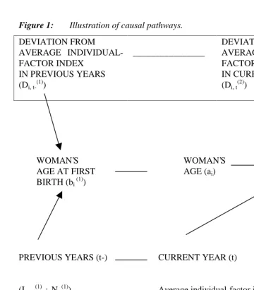
Similarly, a national-factor index N can be produced. It will be the same for all individuals. Because the effects of the various individual and national characteristics differ by birth order, which means that the weights used when creating the indices are different, the indices relevant for second births are referred to as Iav(2) and N(2). This notation is used in Figure 1, which is a sketch of the casual pathways discussed in this section.
Only the characteristics of the women under exposure can be responsible for changes in second-birth rates, not those of, for example, the entire national female population. One reason why these characteristics of the women under exposure may change is that the age of the women increases or decreases. For example, there may have been an increase in the average purchasing power of the exposed women from 1977 to 1997 both because the purchasing power has risen generally, at all ages, and because the women in 1997 are older. Some other factors influenced by age are fecundity and job opportunities. Because there are good reasons for trying to exclude the contribution from age, as explained below, let us now open up for this possibility by redefining the index Iav(2) as an average over women within the entire reproductive age span. More precisely, it could be a weighted average over different age groups between 15 and 40, with age-specific weights reflecting the overall age distribution of the women under exposure in all years under analysis. Women’s age can then be considered as exerting some sort of correction effect: If the women under exposure in a particular year are very old, their real average individual-factor index (i.e. their characteristics of relevance for fertility) is not Iav(2) but something smaller. In other words, a woman’s second-birth rate is in this case given by a combination of Iav(2) and a negative contribution from the age structure. (To avoid confusion, it should perhaps be repeated that none of the fertility determinants mentioned above are available in the data. For the moment, we even ignore the knowledge of individual age. All women are assumed equal, with the same birth rate, determined by the age standardized weighted average of various characteristics the year they are under exposure and the age composition that year. This should be kept in mind also when reading the next paragraphs).
importance here. (In contrast to this, large swings in cohort sizes over many decades have given rise to major changes in the age distribution of the Norwegian population,
Figure 1: Illustration of causal pathways.
DEVIATION FROM DEVIATION FROM
AVERAGE INDIVIDUAL-FACTOR INDEX
________________ AVERAGE INDIVIDUAL-FACTOR INDEX
IN PREVIOUS YEARS IN CURRENT YEAR
(Di, t-(1)
) (Di, t
(2) )
WOMAN’S
WOMAN’S WOMAN’S
SECOND-AGE AT FIRST AGE (ai) BIRTH
BIRTH (bi (1)) RATE
(hi, t(2))
PREVIOUS YEARS (t-) CURRENT YEAR (t)
(Iav,t-(1) + Nt-(1)) Average individual-factor index (Iav,t(2)), based defined as for time t on weighted averages of factors such as: and second births; enrolment, educational level, see to the right income, access to child care
childbearing preferences +
National-factor index (Nt(2)), which is a weighted average of factors such as:
with strong implications for overall mortality.) The most crucial factor is that the age at first birth has increased. Those under exposure for second births in 1997 (and assumed to be younger than 40) were under exposure for a first birth from 1972, or, on average, from the early 1980s. In comparison, those exposed to a second birth in 1977 typically started their reproductive period in the early 1960s, when individual and national-level factors such as those described above were different. For example, fewer were enrolled, and the pill and i.u.d. were not yet available.
Once again, some elaboration may be needed: A woman born, for example, in 1967 was 15 years old in 1982 and her first-birth rate that year reflects people’s characteristics that year, or more precisely the average individual-factor index, based on weights relevant for first rather than second births. In addition, the national-factor index contributes. Surely, only the characteristics of the 15-year olds are relevant, but an age factor will correct for that, as explained above. The next year, when she is 16, her first-birth rate reflects the general characteristics in that year. To simplify, we may say that her age at first birth is determined by a series of national-factor indices and average individual-factor indices over many years before the two years in focus (1977 and 1999). These factors can be symbolized as Iav,t-(1) and Nt-(1) (see Figure 1). The running age while she is under exposure for first birth is of no interest, as all cohorts go through the same ages.
To conclude, a woman in 1997 has a second-birth rate different from that of a woman in 1977 for two main reasons: First, she is likely to have a higher age, because she as a young adult has experienced years with other characteristics at the national level and with another average of various individual factors, and therefore has had a higher age at first birth. Second, the current level of these individual and national variables, with a direct influence on her second-birth rate, is different.
This first pathway can be considered a spill-over from earlier changes in first-birth rates, and one may want to exclude it to get a purer picture of how various current national-level and individual factors influence the second birth in particular. The obvious way to achieve this would be to include some measure of age distribution in the model, along with period. One might perhaps think that the mean age of the women under exposure would be a good candidate, but identification of such period and mean-age effects would be difficult because of a lack of independent variation in these two variables.
adequate approach, because persistent unobserved heterogeneity makes the estimated age effect capture more than the causal effect of age. This is further explained below.
Andersson and Hoem also included duration since previous birth. This is a strong determinant of birth rates. For example, the desire for and the possibility of having an additional child is obviously very weak shortly after birth. Besides, people who have, say, a three-year old child may be more keen to produce a play-mate than those whose youngest child is already seven. (In fact, age and duration may even interact, as women with a high age may be more eager to have their next child fairly soon after the last previous birth because they are more conscious about the possibility of sub-fecundity a few years ahead.) However, duration since previous birth is not so important as a control variable, because it is rather weakly linked with current year (especially for the last two decades of the period of analysis, whereas the sample design creates stronger associations in earlier years). When age is already entered into the model, the additional inclusion of duration has only a small impact on the period effect estimates. (It might seem silly not to include duration in these models that are often referred to as ’duration models’, but it only means that we assume rates to be constant, which we are free to do.)
Such mapping of parity-specific fertility trends by estimating models that only include age, duration and period (although more than the two periods used in the example above, of course) might perhaps seem too mechanistic. However, it can indeed be an important starting-point for further analysis. It may stimulate hypotheses about various driving forces, and indicators of these forces may later, perhaps after having gathered better data, be added to the model to see if the originally estimated period effect is reduced, in which case part of the change over time is explained.
2.2 The Need to Control for Persistent Unobserved Heterogeneity
The essential idea above was that second-birth rates in 1977 are different from those in 1997 partly because women exposed in the latter year tend to have a higher age as a result of a later first birth, and that one may want to remove this contribution. Unfortunately, this is not achieved by simply adding the woman’s age to the period of exposure (plus perhaps duration) in separate models for each parity transition. This is because the woman’s own age at first birth is determined by her own enrolment, childbearing preferences, fecundity and other individual characteristics over the relevant years, rather than the distribution of such factors (in addition, of course, to the national-level factors), and because some of these individual factors are relatively stable and can influence also her current second-birth rate.
More precisely, one may consider the woman’s age at first birth as determined by the national-factor index and the average individual-factor index for the years she has experienced from age 15 (Nt- (1) and It-(1)), plus the individual annual deviations from the latter (Di,t-(1)). These individual deviations in past years must be linked with those during the year under exposure for second birth (Di,t(2)), which must have a bearing on the second-birth rates above and beyond the national-factor index and the average individual-factor index that year. This is illustrated in Figure 1.
we are still picking up changes in behaviour at a lower parity, just as we do in an extremely simple model without age. (Similarly, the women in 1997 are more fertility-prone compared to their contemporaries than those in 1977 also if we fix at a lower age, such as 25. The former are ’ahead of schedule’, whereas the latter have shown mainstream behaviour so far.)
In this study, a joint model for all parity transitions is estimated, with a persistent unobserved heterogeneity factor included. (Such modelling requires, of course, data on more than the two years 1977 and 1997.) This is an attempt to capture the importance of the woman’s position compared to her contemporaries. The unobserved factor is assumed as drawn independently for each woman, from the same approximately normal distribution with zero mean and a variance to be estimated. The factor is further assumed to be constant over the years of follow-up (i.e. reproductive period) for each woman, and influence all her parity transition rates in the same way. The model is specified mathematically in the following section.
This heterogeneity factor does not exactly pick up the Ds defined above, which are time- and parity-dependent, but some sort of ’overall’ deviation from the average characteristics when all the years the woman has lived through and the parity levels she has passed are taken into account (this summation is symbolized by the box in Figure 1). For example, a woman with an exceptionally long school enrolment during young adult years but who is otherwise as others will have a negative heterogeneity factor, as will a woman who remains sub-fecund from an early age. If she also has a very high non-labour income at higher ages, the factor may be more weakly negative or even positive. That will partly depend on whether she is under exposure for a first, second, third or fourth birth at these ages, because the importance of economic resources for the birth rates may in principle differ by parity.
closer to those in the joint model (not shown below). The message is that one should take age into account, but in an appropriate way.
It may be intuitively most easy to understand the importance of persistent unobserved heterogeneity for a second or higher-order parity transition, which has been addressed above. However, similar arguments are also relevant for first-birth rates. For example, as fewer women become mothers in their early 20s, those who are still childless in their late 20s or 30s will to a lesser extent be among the low-fertility prone, which will push first-birth rates at these ages up.
To make it even more complex, a selection mechanism corresponding to the last mentioned is relevant also for higher-order births, in addition to that already explained: If we, for example focus on one-child mothers at age 30 with a first birth 4 years before, and compare their second-birth rates in 1977 and 1997, these rates will differ not only because a first-birth at age 26 was late for the 1947 cohort and mainstream behaviour for the 1967 cohort, but also because those who are still one-child mothers after 4 years must be a more fertility-prone group in 1997, when recent second-birth rates have been generally lower than they were 20 years before. In light of this, the separate modelling should give biased estimates of time trends already from the mid-1960s, when the second-birth rates started to fall (whereas the first-birth rates did not fall until the early 1970s).
Finally, it may be important to point out that the inclusion of unobserved heterogeneity is more than a mechanical search for a better model fit. It certainly improves the fit, but an equally good fit, or even better, can be achieved with a model without unobserved heterogeneity if age, duration and period profiles are sufficiently fine-tuned (by using e.g. a larger number of nodes in the spline) and complex interactions are allowed. However, the joint model with unobserved heterogeneity has the advantage of being more parsimonious and theoretically motivated.
3. The Estimation Procedure in Detail
The register data used for the estimation include all women born 1936-81 who have been assigned a Norwegian personal identification number, i.e. who have lived in Norway some time after 1960. Birth histories up to 1997, established from the Central Population Register, are virtually complete for these women. Date of death or last emigration, if any, is also recorded.
in 1967). For example, the estimated time trend between 1960 and 1965 will be based on observed behaviour among women in their teens or 20s, whereas that estimated for the late 1970s, the 1980s and the 1990s will be based on all reproductive ages up to 40. This means that there will be a relatively large variance in the trend estimates for these early years for transitions that are rare at low ages, such as fourth births. More importantly, one will get a wrong impression of the trends if they are markedly dependent on age. Such a period-age interaction does appear to exist: Separate models for each parity transition reveal, on the whole, that the downward trend before the mid-1970s was least sharp for the highest ages observed (not shown). Thus, a less pronounced decline would probably have been estimated if a larger age span had been available for the first part of the period under study. As a quantitative illustration of this, additional calculations were made with the 1936-40 cohorts excluded, which resulted in a decline from the mid-1960s to the mid 1970s which was roughly 1/3 sharper than estimated with these cohorts included (not shown). This is a substantial bias, but it is possible that the opposite, namely inclusion of cohorts before 1936, might have had a smaller impact (in the opposite direction, of course). In support of this, there seems to be a diminishing strength of the period-age interaction as age increases. Fortunately, a similar bias cannot possibly explain the increase in second- and higher-order births after the mid-1970s, which is in focus of this study, because all ages contribute in the estimation for this period.
To reduce computer time, a 33% random sample was drawn from the register file. The sample is still huge by most standards, and the trends are smooth and very similar to those obtained with other methods and a full sample.
Birth rate models were estimated in the aML software (Lillard and Panis 2000), which uses a likelihood maximization procedure based on analytic first derivatives and the BHHH search algorithm. As a first step, models were estimated separately for first, second, third and fourth births. Separate models were also estimated for first births among women aged 15-30 and for those aged 30-40, to achieve comparability with Andersson’s work (Note 3). The follow-up was from age 15 to 30, or from 30 to 40, in the first-birth models, and from previous birth to age 40 in the higher-order birth models, unless it was censored at a lower age because of death or emigration, or because the end of 1997 (which is the last day the biographies cover) was reached.
In mathematical terms, the specifications are as follows:
log h(1y)(a, y) = 0(1y) + 1(1y) A(a,vA 1,v2) + 2(1y) Y(y,tY 1,t2, … t14,t15)
log h(1o)(a, y) = 0(1o) + 1(1o) A(a,vA 3) + 2(1o) Y(y,tY 1,t2, … t14,t15)
log h(2)(a,d,y) = 0 (2)
+ 1 (2)
A
A(a,v4) + 2 (2)
Y
Y(y,t1,t2, … t14,t15) ++ 3 (2)
D
D((d,z1,z2,z3,z4)
log h(3)(a,d,y) = 0(3) + 1(3) A(a,vA 4) + 2(3) Y(y,tY 1,t2, … t14,t15) ++ 3(3) D((d,zD 1,z2,z3,z4)
log h(4)(a,d,y) = 0(4) + 1(4) A(a,vA 4) + 2(4) Y(y,tY 1,t2, … t14,t15) ++ 3(4) D((d,zD 1,z2,z3,z4)
where h is a birth rate and (1), (2), (3), and (4) are symbols for first, second, third and fourth births, respectively. 1y refers to the first-birth model for the young ages 15-30, and 1o for the older ages 30-40.
In these equations, 0 is a constant, and AA(a,v1,v2) is a piecewise linear spline transformation of age, with nodes at v1=20 years and v2 =25 years. It is defined as a column vector whose transpose is
A
At= (min[a,v1], max[0,min[a-v1, v2-v1]], max[0,a-v2]).
1 is the corresponding row vector of effects. YY(y,t1,t2, … t14,t15 ) is the spline transformation of year, with 15 nodes at 1960, 1962.5, 1965, … 1995. 2 is the corresponding row vector of effects. The model for age 30-40 is similar, except that there is an age spline AA(a,v3), with a node at v3=35 years.
Also AA(a,v4), which is included for second- and higher-order births, is an age spline with one node at v4 = 35 years, whereas DD (d, z1,z2,z3,z4) is a duration spline with four nodes at z1 = 2 years, z2 = 4 years, z3 = 6 years, and z4 = 8 years.
The next step was to add a random factor to all five equations and estimate them simultaneously:
log h(1y)( a,y) = 0 (1y)
+ 1 (1y)
A
A(a,v1,v2) + 2 (1y)
Y
Y(y,t1,t2, … t14,t15) +
log h(1o)( a,y) = 0(1o) + 1(1o) A(a,vA 3) + 2(1o) Y(y,tY 1,t2, … t14,t15) +
log h(3)(a,d,y) = 0(3) + 1(3) A(a,vA 4) + 2(3) Y(y,tY 1,t2, … t14,t15 ) ++ 3(3) D((d,zD 1,z2,z3,z4) +
log h(4)(a,d,y) = 0(4) + 1(4) A(a,vA 4) + 2(4) Y(y,tY 1,t2, … t14,t15 ) ++ 3(4) D((d,zD 1,z2,z3,z4) +
The factors for the different individuals are assumed to be independent identically distributed with mean 0 and variance σ2. A woman's -factor sticks to her throughout her reproductive period, and influences all her parity transition rates in the same way.
For each person, aML calculates a joint likelihood for the outcomes, conditional on different values of the heterogeneity factor. Next, it is integrated numerically over these values and summed over all individuals. The resulting likelihood is the one to be maximized. The values of the heterogeneity factor (so-called support points) and the corresponding weights are chosen to approximate the normal distribution (the so-called Gauss-Hermite approximation). The number of support points is chosen by the user. The results shown below are from calculations based on 15 support points, which is obviously sufficient. Whereas the use of ten support points gave results slightly different from those obtained with four support points, there was no further change when another five support points were added.
Variances were generally small with this huge data set, so all increases and decreases mentioned below were significant at the usual levels.
4. Results
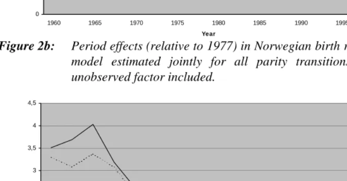
Period effect estimates are illustrated in Figures 2a and 2b for the separate models and the joint model, respectively. The curves are anchored in 1 in 1977, to make them more easily comparable with those shown by Andersson. (More precisely, birth rates are first predicted for all node years for an arbitrarily chosen age and duration. Each of these rates are then divided by the rate for the 1977 node). The standard deviation σ of the random term was estimated to be 0.893 (with a standard error of 0.009).
Of course, exactly the same trends appear in Figure 2a as in similar graphs based on models where all regressors are categorized, as in Andersson’s work.
Figure 2a: Period effects (relative to 1977) in Norwegian birth rates, according to models estimated separately for each parity transition
Figure 2b: Period effects (relative to 1977) in Norwegian birth rates, according to a model estimated jointly for all parity transitions, with a common unobserved factor included.
0 0,5 1 1,5 2 2,5 3 3,5 4
1960 1965 1970 1975 1980 1985 1990 1995
Year
R
e
lat
ive r
a
te First birth, age 15-30
Second birth Third birth Fourth birth
0 0,5 1 1,5 2 2,5 3 3,5 4 4,5
1960 1965 1970 1975 1980 1985 1990 1995
Year
R
e
la
tiv
e
r
a
te First birth, age 15-30
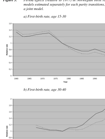
Figure 3: Period effects (relative to 1977) in Norwegian birth rates, according to models estimated separately for each parity transitions, and according to a joint model.
a) First-birth rate, age 15-30
b) First-birth rate, age 30-40
0 0,2 0,4 0,6 0,8 1 1,2 1,4 1,6
1960 1965 1970 1975 1980 1985 1990 1995
Year
Re
la
ti
v
e
r
a
te
Separate model Joint model
0 0,2 0,4 0,6 0,8 1 1,2 1,4 1,6 1,8 2
1960 1965 1970 1975 1980 1985 1990 1995
Year
Re
la
ti
v
e
r
a
te
c) Second-birth rate
d) Third-birth rate
0 0,5 1 1,5 2 2,5
1960 1965 1970 1975 1980 1985 1990 1995
Year
R
e
la
ti
v
e
r
a
te
Separate model Joint model
0 0,5 1 1,5 2 2,5 3 3,5 4
1960 1965 1970 1975 1980 1985 1990 1995
Re
la
ti
v
e
r
a
te
e) Fourth-birth rate
It is seen in Figure 3 that the increase in the second-birth rates is restricted to the separate model. According to the joint-model approach, there is actually a decline: The second-birth rate is 5% lower in 1997 than in 1977, and more than 10% lower in two of the intermediate years.
Third-and fourth birth rates are rising both in the joint-model approach and the separate-model approach, but there is a substantial difference in magnitude: The increase in the third-birth rate from 1977 to 1997 according to the joint-model approach is slightly less than half of what it is according to the separate model, and the increase in the fourth-birth rate is slightly less than one-third.
Put differently, when Norwegian higher-order birth rates at a given age increase substantially over the 20-year period in Andersson’s plots, it is to a large extent because those who have reached so high parity at this age in the most recent years score higher on some unobserved persistent characteristics associated with high fertility.
The joint-model approach also shows more of a decline in first-birth rates after the mid- 1970s, and it shows a stronger downward trend before the mid-1970s for all parity transitions, as expected.
0 0,5 1 1,5 2 2,5 3 3,5 4 4,5
1960 1965 1970 1975 1980 1985 1990 1995
Year
Re
la
ti
v
e
r
a
te
5. Conclusion
When simple period effect estimates are wanted for each parity transition, on the basis of data on dates of birth exclusively, it can be argued that the joint-model approach is more satisfactory than the separate-model approach used by Andersson and, previously, Hoem. This is because the period effects in the Andersson-Hoem models capture some individual fertility differentials that have little to do with the periods in focus, but are linked with earlier changes in lower-order parity transitions. The main argument for trying to take age into account, rather than simply calculating annual occurrence-exposure rates for different parities, is that the trends in such rates would reflect also the changes in lower-parity transition in the (immediate) past. However, one does not get rid of such contributions by including age as in the Andersson-Hoem approach. One contribution of this kind is merely substituted by another.
Some important differences do show up in the estimates, which supports the conclusion from a recent study of education effects that the more cumbersome simultaneous modelling can indeed be more than a futile methodological snobbery (Kravdal 2001). However, one should hesitate to consider it a huge step forward. Except for the second births, the directions of the time trends are the same according to the joint-model approach as according to the Andersson-Hoem approach, but the changes are less pronounced. Thus, there is still a need to find good reasons for an upsurge in third and fourth births in Norway from the mid-1970s. (In fact, also an abrupt stabilization, after more than a decade of steep downhill movement, would need explanation). Such an upsurge would probably have appeared also in a similar estimation for Sweden, where the changes in the birth rates were no less pronounced than those in Norway according to the separate-model approach.
The picture is different for second births: The joint-model estimates reveal that second-birth rates have fallen very modestly in Norway after the mid-1970s, rather than increased.
Similarly, there may be no real increase in second-birth rates in Sweden, except for the first 2-3 years after first birth, when the ‘speed premium’ is likely to have been the driving force. According to Andersson, the increase at later durations was of the same size in Sweden as in Norway, so it might well have been wiped out in a joint-model approach.
she had her last previous birth (i.e. when she attained that parity)’. This variable is constant over the spell. The period effect estimates turned out to be quite similar to those obtained with the unobserved-heterogeneity model (Note 4).
It might also be worthwhile to try other specifications of the unobserved heterogeneity. The only alternative that was checked here was to include different, but correlated, heterogeneity terms for parity transitions up to and after second birth - the theoretical justification being that higher-parity transitions reflect more of a quantum and less of a timing or spacing decision, and may depend on other factors. This gave quite different period effects for fourth births, but otherwise very similar results.
6. Acknowledgements
Notes
1. This development in the birth rates among women who have already had their first child is consistent with quantum changes reported elsewhere. For example, Kravdal (2001) pointed out that cohort fertility in Norway has been steadily reduced for those born after the Depression, especially because a growing proportion have refrained from having more than two children, but that the reduction has been very modest for the youngest cohorts. There has been some reduction also in the proportion who have had a second child.
2. Of course, both the lower cohort fertility and the higher age at first, and thus later, births contributed to the reduction of total fertility in the 1970s in both countries. Moreover, the stabilization or upturn of first-birth rates from the mid 1980s was an important factor behind the rising total fertility: Generally, when age at first birth has increased for some time, more and more women enter the high 20s and the 30s as childless, which contributes to increase the number of births at these ages, unless first-birth rates at these ages are reduced (in which case also the proportion of childless would escalate). When there is not at the same time a further reduction of first births among the younger adults, the first-birth contribution (in absolute terms) to total fertility will show an upward trend.
3. This split at age 30 may be considered inelegant because it introduces a discontinuity in the age profile. Fortunately, it has no consequences for the estimated effects of period for second and higher-order births in the joint model described below. For example, one could hardly see a change in the period effect estimates corresponding to 1997 when the model was estimated without such a split (i.e. the h(1o) contribution dropped and the h(1y) contribution extended to the 15-40 age interval with two additional age nodes at 30 and 35, but still without any age-period interaction).
References
Andersson, G. (2002). ”Fertility developments in Norway and Sweden since the early 1960s.” Demographic Research online at www.demographic-research.org/ Volumes/Vol6/4.
Hoem, J.M. (1990). ”Social change and recent fertility decline in Sweden.” Population and Development Review 16: 73 5-748.
Hoem, J.M. (1993) ”Classical demographic methods of analysis and modern event-history techniques.” IUSSP: 22nd International Population Conference Montreal, Canada, Volume 3: 281-291.
Kravdal, Ø. (2001). “The high fertility of college educated women in Norway: An artefact of the separate modelling of each parity transition.” Demographic Research online at www.demographic-research.org/ Volumes/Vol5/6.
Lillard, L, and C.W.A. Panis. (2000). aML Multilevel Multiprocess Statistical Software. Release 1.0. EconWare, Los Angeles, California