Superconvergence analysis of multistep collocation method for delay functional integral equations

(1)

Superconvergence analysis of multistep collocation method for

de-lay Volterra integral equations

P. Darania

Department of Mathematics, Faculty of Science, Urmia University, P.O.Box 165, Urmia-Iran.

Abstract In this paper, we will present a review of the multistep collocation method for Delay Volterra Integral Equations (DVIEs) from [4] and then, we study the supercon-vergence analysis of the multistep collocation method for DVIEs. Some numerical examples are given to confirm our theoretical results.

Keywords. Delay integral equations, Multistep collocation method, Convergence and superconvergence analysis.

2010 Mathematics Subject Classification. 65L05, 34K06, 34K28.

1. _Introduction

Many special cases of the diﬀerential and integral delay equation, can be encoun-tered in applications: absorption of light by interstellar matter [1], analytic number theory [8], collection of current by the pantograph of an electric locomotive [9], nonlin-ear dynamical system [5], probability theory on algebraic structures [11], Cherenkov radiation [9], continuum mechanics [10], and the theory of dielectric materials [7]. Moreover, delay equation is an interesting example of a functional equation with a variable delay: suﬃciently complicated to provide a clue to the behavior of more general classes of such equations, but also simple enough to be tractable by relatively straightforward means. For more detail see [7] and the references therein.

Consider the Volterra functional integral equation with delay functionθ(t),

y(t) =       

g(t) + ∫ t

t0

k1(t, s, y(s))ds+

∫ θ(t)

t0

k2(t, s, y(s))ds, t∈[t0, T],

ϕ(t), t∈[θ(t0), t0),

(1.1)

wherek1∈C(D×R), D={(t, s) :t0≤s≤t≤T}andk2is assumed to be continuous

inDθ×R, Dθ={(t, s) :θ(t0)≤s≤θ(t)}, withI= [t0, T] andϕ: [θ(t0), t0]→Rand g: [t0, T]→Rare at least continuous on their domains.

The delay functionθsatisfy in the following conditions:

Received: 20 June 2016 ; Accepted: 1 January 2017.

(2)

(D1) θ(t) =t−τ(t), withτ(t)≥τ0>0 for t∈I; (D2) θis strictly increasing on I;

(D3) τ∈Cd(I) for somed≥0.

We will refer to the functionτ=τ(t) as the delay.

Definition 1.1. The points{ξµ: µ≥0}generated by the recursion

θ(ξµ+1) =ξµ+1−τ(ξµ+1) =ξµ, µ= 0,1, ..., ξ0=t0,

are called the primary discontinuity points associated with the lag function θ(t) =

t−τ(t).

Condition (D2) ensures that these discontinuity points have the (uniform) separa-tion property

ξµ−ξµ₋1=τ(ξµ)≥τ0>0, for allµ≥1.

Theorem 1.2. Assume that the given functions in

y(t) =       

g(t) + ∫ t

t0

k1(t, s)y(s)ds+ ∫ θ(t)

t0

k2(t, s)y(s)ds, t∈[t0, T],

ϕ(t), t∈[θ(t0), t0),

(1.2)

are continuous on their respective domains and that the delay functionθ satisﬁes the above conditions (D1)-(D3). Then for any initial functionϕ∈C[θ(t0), t0]there exists a unique (bounded)y∈C(t0, T]solving the Volterra functional integral equation (1.1) on (t0, T] and coinciding with ϕ on [θ(t0), t0]. In general, this solution has a ﬁnite (jump) discontinuity att=t0:

lim

t→t+₀

y(t)̸= lim

t→t−₀

y(t) =ϕ(t0).

The solution is continuous att=t0 if, and only if, the initial function is such that

g(t0)− ∫ θ(t0)

t0

k2(t0, s)ϕ(s)ds=ϕ(t0).

Proof. See [2].

It is well known that these equations typically have discontinuity in the solution or its derivatives at the initial point of integration domain. This discontinuity propagated along the integration interval giving rise to subsequent points, called singular points, which can not be determined priori and the solution derivatives in these points are smoothed out along the interval. Most of the known numerical methods for this type of equations are generally very sensitive to the singular points and therefore must have a process that detects these points and insert them into the mesh to guarantee the required accuracy.

(3)

with delay arguments. P. Darania [4], had considered the nonlinear Volterra integral equations with constant delaysθ(t) =t−τ, τ >0, of the form

y(t) =   

g(t) + (V y)(t) + (Vτy)(t), t∈I= [0, T],

ϕ(t), t∈[−τ,0),

(1.3)

where

(V y)(t) = ∫ t

0

k1(t, s, y(s))ds, (1.4)

(Vτy)(t) =

∫ t₋τ

0

k2(t, s, y(s))ds, (1.5)

and the given functions,ϕ: [−τ,0]→R, g:I→R, k1:D×R→R, D={(t, s) : 0≤

s≤t ≤T} and k2 :Dτ×R →R, Dτ =I×[−τ, T −τ] are at least continuous on

their domains.

In the present paper, we are brieﬂy introduced the new families of multistep collo-cation method which has presented in [4, 3]. Also, we analyze the superconvergence analysis of the multistep collocation method when used to approximate smooth solu-tions of delay integral equasolu-tions. Some numerical examples are given to conﬁrm our theoretical results.

2. Preliminaries

Here, we recall the multistep collocation method that have been introduced in [4,3].

2.1. Multistep collocation method. Lettn=nh, (n= 0, . . . , N, tN =T, h=

τ ˜

r for som ˜r∈N) deﬁne a uniform partition forI= [0, T], and let ΩN :={0 =t0< t1<· · ·< tN =T}, σ0:= [t0, t1], σn := (tn, tn+1] (1≤n≤N−1). With a given mesh

ΩN, we associate the set of its interior points,ZN :={tn :n= 1, . . . , N−1}. For a

ﬁxedN ≥1 and, for given integerm≥1, the piecewise polynomial spaceS_m(−₋1)₁(ZN)

is deﬁned by

S_m(−₋1)₁(ZN) :={u:u|σn=uh∈Πm−1, 0≤n≤N−1},

where Πm₋1 denotes the set of (real) polynomials of a degree not exceedingm−1.

Letuh=u|σn, u∈S

(−1)

m−1(ZN), for allt∈σn, we have uh(tn+sh) =

r−1

∑

k=0

φk(s)yn−k+ m

∑

j=1

ψj(s)Un,j, s∈[0,1], n=r, . . . , N−1, (2.1)

whereUn,j=uh(tn,j), yn₋k =uh(tn₋k) and

φk(s) = m

∏

i=1 s−ci

−k−ci · r_∏−1 i=0 i̸=k

s+i

−k+i, ψj(s) = r_∏−1 i=0

s+i cj+i·

m

∏

i=1 i̸=j

s−ci cj−ci

(4)

Remark 2.1. In the following, we assume that the initial functionϕ(t) is such that

g(0)− ∫ ₋τ

0

k2(0, s)ϕ(s)ds=ϕ(0).

The collocation solutionuhwill be determined by imposing the condition thatuh

satisﬁes the integral equation (1.3) on the ﬁnite setXN ={tn,j=tn+cjh}

uh(t) =

  

g(t) + (V uh)(t) + (Vτuh)(t), t∈[0, T],

ϕ(t), t∈[−τ,0),

(2.3)

where{cj}mj=1, 0≤c1<· · ·< cm≤1, the set of collocation parameters. After some

computations, the exact multistep collocation method is obtained by collocating both sides of (2.3) at the pointst=tn,jforj= 1,2, . . . , mand computingyn+1=uh(tn+1):

    

Un,j=Dn,j, j= 1,2, . . . , m,

yn+1= r−1

∑

k=0

φk(1)yn−k+ m

∑

j=1

ψj(1)Un,j, n=r, r+ 1, . . . , N −1,

(2.4)

whereDn,j =D(tn,j) and

D(tn,j) =g(tn,j) +

  

(V uh)(tn,j) + Φ(tn,j), tn,j−τ <0,

(V uh)(tn,j) + (Vτuh)(tn,j), tn,j−τ ≥0,

(2.5)

Φ(tn,j) =

∫ tn,j−τ

0

k2(tn,j, s, ϕ(s))ds, j = 1,2, . . . , m, n= 0,1, . . . ,˜r−1, (2.6)

and fortn,j−τ <0, we have

(Vτuh)(tn,j) = −h

[∫ 1

cj

k2(tn,j, tn−r˜+sh, ϕ(tn−r˜+sh))ds

+

−1

∑

i=n₋r˜+1

∫ 1

0

k2(tn,j, ti+sh, ϕ(ti+sh))ds

]

,

(2.7)

and fortn,j−τ ≥0, we get

(Vτuh)(tn,j) = h

[_n₋_˜_r₋₁ ∑

i=0

∫ 1

0

k2(tn,j, ti+sh, uh(ti+sh))ds

+ ∫ cj

0

k2(tn,j, tn−˜r+sh, un−r˜(tn−˜r+sh))ds

]

,

(5)

and

(V uh)(tn,j) = h n∑−1

i=0

∫ 1

0

k1(tn,j, ti+sh, uh(ti+sh))ds

+h

∫ cj

0

k1(tn,j, tn+sh, uh(tn+sh))ds.

(2.9)

By using quadrature formulas with the weights wl and nodes dl, l = 1, . . . , µ1, for

integrating on [0,1], and the weightswj,l and nodesdj,l, l= 1, . . . , µ0for integrating

on [0, ci], with positive integersµ0 andµ1, one can write

    

Yn,j= ¯Dn,j, j= 1,2, . . . , m,

yn+1= r−1

∑

k=0

φk(1)yn−k+ m

∑

j=1

ψj(1)Yn,j, n=r, r+ 1, . . . , N−1,

(2.10)

where ¯

D(tn,j) =g(tn,j) + ( ¯V uh)(tn,j) + ( ¯Vτuh)(tn,j), (2.11)

( ¯V uh)(tn,j) = h n_∑−1

i=0 µ1

∑

l=1

wlk1(tn,j, ti+dlh, Pi(ti+dlh))

+h µ0

∑

l=1

wj,lk1(tn,j, tn+dj,lh, Pn(tn+dj,lh)),

(2.12)

and fortn,j−τ <0, we have

( ¯Vτuh)(tn,j) = −h

( ₋₁ ∑

i=n−˜r+1 µ1

∑

l=1

wlk2(tn,j, ti+dlh, ϕ(ti+dlh))

+

µ1

∑

l=1

¯

wj,lk2(tn,j, tn−˜r+ξj,lh, ϕ(tn−r˜+ξj,lh))

)

,

(2.13)

and fortn,j−τ ≥0, we get

( ¯Vτuh)(tn,j) = h

(_n₋_˜_r₋₁ ∑

i=0 µ1

∑

l=1

wlk2(tn,j, ti+dlh, Pi(ti+dlh))

+

µ0

∑

l=1

wj,lk2(tn,j, tn−˜r+dj,lh, Pn−˜r(tn−r˜+dj,lh))

)

,

(2.14)

andξj,l :=cj+ (1−cj)dl, w¯j,l := (1−cj)wl, j= 1, . . . , m, l= 1, . . . , µ1. Also,

the discretized multistep collocation polynomial, denoted by

Pn(tn+sh) = r−1

∑

k=0

φk(s)yn−k+ m

∑

j=1

(6)

(2.15)

For more detail see [4].

2.2. Convergence. Letuh ∈ S

(₋1)

m−1(ZN) denote the (exact) collocation solution to

(1.3) deﬁned by (2.4). In convergence analysis, we consider the linear test equation

y(t) =   

g(t) + ∫ t

0

k1(t, s)y(s)ds+ ∫ t−τ

0

k2(t, s)y(s)ds, t∈I, ϕ(t), t∈[−τ,0),

(2.16)

wherek1∈C(D) andk2∈C(Dτ).

Theorem 2.2. Let the given functions in (2.16) satisfyg∈Cp₍_I₎_{, k1}_∈_Cp₍_D₎_{, k2}_∈

Cp₍_D

τ), ϕ∈Cp([−τ,0]), and fort∈[0, τ]the integral

Φ(t) := ∫ t₋τ

0

k2(t, s)ϕ(s)ds, (2.17)

is known exactly. Also, suppose that the starting error is

∥y−uh∥_∞,[0,tr]=O(h

p₎_, _(2.18)

and

ρ(A)<1, (2.19)

wherep=m+randρdenotes the spectral radius and

A=

[

0(r−1)×1 Ir−1

φr−1(1) φr−2(1), ..., φ0(1)

]

. (2.20)

Then for all suﬃciently small h = τ_r_˜, (˜r ∈ N) the constrained mesh collocation solutionuh∈S

(−1)

m−1(ZN)to (2.16), satisﬁes

∥ E ∥∞≤Chp, (2.21)

where E(t) = y(t)−uh(t) be the error of the exact collocation method (2.11) and C is positive constant not depending on h. This estimate holds for all collocation parameters{cj} with 0≤c1<· · ·< cm≤1.

Proof. See [4].

Remark 2.3. [3]. The starting valuesy1, y2, . . . , yr,needed in (2.4) and (2.10), may

be obtained by using a suitable starting procedure, based on a classical one step method has uniform convergence order ofp.

Theorem 2.4. Let the assumptions of Theorem2.2hold, except that the integrals

Φ(t) = ∫ t−τ

0

k2(t, s)ϕ(s)ds, t=tn,j, n= 0,1, ...,˜r−1,

are now approximated by quadrature formulas Φ(¯ t), with corresponding quadrature errorsE0(t) := Φ(t)−Φ(¯ t), such that

(7)

for some q > 0. Then the collocation solution uh ∈ S (−1)

m₋1(ZN) satisﬁes, for all suﬃciently smallh >0,

∥ E ∥∞≤Chp, (2.23)

withp:= min{m+r, q}, whereC are ﬁnite constants not depending onh.

Proof. See [4].

3. Superconvergence

In this section, we analyze the superconvergence of the multistep collocation method when used to approximate smooth solutions of delay integral equations.

By the following theorem, we obtain local superconvergence in the interior points

ZN.

Theorem 3.1. Suppose that the hypothesis of Theorem2.2hold withp= 2m+r−1

and the collocation parametersc1, ..., cm are the solution of system

    

cm= 1,

1 i+1 −

r−1

∑

k=0

βk(−k)i− m

∑

j=1

γj(cj)i= 0, i=m+r, ...,2m+r−2, (3.1)

where

βk =

∫ 1

0

φk(s)ds, γj=

∫ 1

0

ψj(s)ds. (3.2)

Also, suppose that the delay integral

Φ(t) = ∫ t−τ

0

k2(t, s, ϕ(s))ds, (3.3) can be evaluated analytically and ifh=τ

˜

r is suﬃciently small. Then

max

1≤n≤N|E(tn)| ≤Ch

p_. _(3.4)

Proof. Without loss of generality, we assume that T =tN =M τ for some M ∈N.

The collocation equation (2.16) may be written in the form

uh(t) =−δ(t) +g(t) +

∫ t

0

k1(t, s)uh(s)ds+

∫ t₋τ

0

k2(t, s)uh(s)ds, t∈I, (3.5)

where the defect functionδvanishes onXN

δ(tn,j) = 0. (3.6)

Also, we haveδ(t) = 0 fort <0. The collocation errorE=y−uh solves the integral

equation [2,6]

E(t) =δ(t) + ∫ t

0

k1(t, s)E(s)ds+F(t), t∈I, (3.7)

where

F(t) = ∫ t₋τ

0

(8)

Fort∈[0, τ], we haveF(t) = 0 and so the error equation (3.7) reduces to a classical Volterra equation, which is unique solution given by [2,6]

E(t) =δ(t) + ∫ 1

0

R1(t, s)δ(s)ds, (3.9)

where R1 denotes the resolvent kernel associated with the given kernel k1. As T =

M τ for some positive integer M, we may set ξµ :=µτ, µ = 0, ..., M, and then for t ∈ [ξµ, ξµ+1], 1 ≤µ ≤ M −1 the collocation error E(t) governed by (3.7) can be

expressed in the form [6,2]

E(t) =δ(t) +

µ

∑

i=0

∫ t−iτ

0

Rn,i(t, s)δ(s)ds, (3.10)

where the functionRn,i(t, s) depend on the given kernel functionski(t, s), i= 1,2.

Fort=tn∈[ξµ+h, ξµ+1], and h= τ_r_˜ for some ˜r∈N, we obtain

E(tn) =δ(tn) +h µ

∑

i=0 n₋_∑i˜r₋1

ν=0

∫ 1

0

Rn,i(tn, tν+sh)δ(tν+sh)ds. (3.11)

Now, let us consider the quadrature formula ∫ 1

0

f(s)ds≈ r−1

∑

k=0

βkf(−k) + m

∑

j=1

γjf(cj),

for the computation of the integrals in (3.11), we have

E(tn) = δ(tn) +h µ

∑

i=0 n−∑ir˜−1

ν=0

[_r₋₁ ∑

k=0

βkRn,i(tn, tν−k)δ(tν−k)

+

m

∑

j=1

γjRn,i(tn, tν,j)δ(tν,j)

 +h

µ

∑

i=0 n−∑ir˜−1

ν=0

En,i,ν,

(3.12)

whereEn,i,ν the corresponding error terms. The hypothesiscm= 1 assures thattν₋k

are collocation points for eachν. Since the defect function vanish in the collocation points, we haveδ(tν,j) =δ(tν₋k) = 0, hence

E(tn) =h µ

∑

i=0 n−∑ir˜−1

ν=0

En,i,ν, 0≤µ < n≤µ+ 1≤M, M τ =T. (3.13)

The quadrature errors in (3.13) can be bounded by |En,i,ν| ≤Ch2m+r−1 with some

ﬁnite constantCnot depending onh, (see [3] and [6]). Finally, becauseM τ =Mrh˜ =

T =N h, we obtain max

1≤n≤N|E(tn)| ≤Ch

2m+r−1_.

(9)

Finally, we comment on the extension of the results in Theorem3.1to the nonlinear case. Instead of (3.7), the equation for the multistep collocation errorE now has the form

E(t) =δ(t) + ∫ t

0

{k1(t, s, y(s))−k1(t, s, uh(s))}ds+F(t), t∈I, (3.14)

where

F(t) = ∫ t−τ

0

{k2(t, s, y(s))−k2(t, s, uh(s))}ds, t∈[τ, T]. (3.15)

Under appropriate diﬀerentiability and boundness conditions for k1 and k2, we

obtain

ki(t, s, y(s))−ki(t, s, uh(s)) = ∂ki

∂y(t, s, y(s))E(s) +

1 2

∂2_k i

∂y2(t, s, zi(s))E 2₍_s₎_,

where zi is between y and uh. The global convergence ofV(uh), Vτ(uh),V¯(uh) and

¯

Vτ(uh) has already been establish [4]. So, we know that∥ E2 ∥∞= O(h2(m+r)) for

any{cj}.

4. _{Presentation of results}

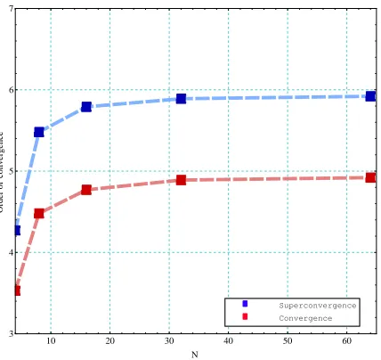
In this section, two examples will be investigated to conﬁrm our theoretical results. We consider the multistep collocation method withm= 2, r= 3, given by Examples

4.1and 4.2with the following choices of the collocation abscissas: (c1, c2) = (0.7,1) and from system (3.1), (c1, c2) = (21₃₈,1). The method have respectively orderp= 5 (convergence) and p = 6 (superconvergence). The observed orders of convergence are computed from the maximum errors at the grid points. The starting values have been obtained from the known exact solutions. All computations are performed by the Mathematicar software.

Example 4.1. Consider the linear DVIEs as

y(t) =g(t) + ∫ t

0

(s+t+ 1)y(s)ds+ ∫ t₋1

2

0

(s+t2+ 4)y(s)ds, t∈[0,1],

whereg(t) such that the exact solution isy(t) = sint.

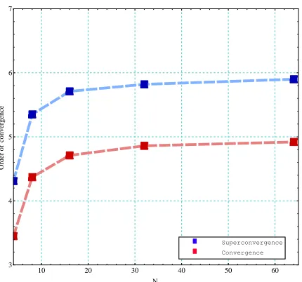
Example 4.2. Consider the nonlinear DVIEs as

y(t) =g(t) + ∫ t

0

2 cos(t−s)y2(s)ds+ ∫ t−1

2

0

2 sin(t−s)y2(s)ds, t∈[0,1],

whereg(t) such that the exact solution isy(t) =et_.

(10)

Table 1. Maximum errors ∥y −uh∥_∞ for r = 3 and m = 2 in

Example4.1.

c1= 0.7, c2= 1 c1=21₃₈, c2= 1

N ||y−uh||∞ ||y−uh||∞

4 2.12002×10−6 ₃_.₈₇₈₈₈_×₁₀−7

8 1.83053×10−7 ₂_.₀₀₀₀₀_×₁₀−8

16 8.19697×10−9 ₄_.₄₅₁₁₄_×₁₀−10

32 2.99995×10−10 ₈_.₀₂₈₃₆_×₁₀−12

64 1.00999×10−11 ₁_.₃₅₂₂₅_×₁₀−13

Figure 1. Orders of convergence of uh for r = 3 and m = 2 in

Example4.1.

10 20 30 40 50 60

3 4 5 6 7

N

Order

of

convergence

Convergence Superconvergence

(the orders of convergence and superconvergence arep=m+r andp= 2m+r−1, respectively).

5. _Conclusion

(11)

Table 2. Maximum errors ∥y −uh∥_∞ for r = 3 and m = 2 in

Example4.2.

c1= 0.7, c2= 1 c1=21₃₈, c2= 1

N ||y−uh||∞ ||y−uh||∞

4 1.15904×10−4 ₅_.₀₆₈₅₀_×₁₀−5

8 1.22162×10−5 ₂_.₅₄₁₂₆_×₁₀−6

16 5.89844×10−7 ₆_.₁₉₃₉₆_×₁₀−8

32 2.23937×10−8 ₁_.₁₈₁₈₀_×₁₀−9

64 7.68051×10−10 ₂_.₀₇₈₃₈_×₁₀−11

Figure 2. Orders of convergence of uh for r = 2,3 andm = 2 in

Example4.2.

10 20 30 40 50 60

3 4 5 6 7

N

Order

of

convergence

Convergence Superconvergence

of collocation parameters.

Acknowledgment

(12)

References

[1] V.A. Ambartsumian, On the ﬂuctuation of the brightness of the Milky Way, Doklady Akad. Nauk USSR,44(1944), 223–226.

[2] H. Brunner,Collocation Methods for Volterra Integral and Related Functional Equations, Cam-bridge Monographs on Applied and Computational Mathematics, 15, Cambridge University Press, Cambridge, 2004.

[3] D. Conte and B. Paternoster, Multistep collocation methods for Volterra integral equations, Appl. Numer. Math.,59(2009), 1721–1736.

[4] P. Darania,Multistep collocation method for nonlinear delay integral equations, Sahand Com-munications in Mathematical Analysis (SCMA),3(2016), 47–65.

[5] G.A. Derfel,Kato problem for functional-diﬀerential equations and diﬀerence Schrodinger op-erators, Operator Theory: Advances and Applications,46(1990), 319-321.

[6] V. Horvat,On collocation methods for Volterra integral equations with delay arguments, Math-ematical Communications,4(1999), 93–109.

[7] A. Iserles,On the generalized pantograph functional-diﬀerential equation, Euro. Jnl of Applied Mathematics,4(1993), 1–38.

[8] K. Mahler,On a special functional equation,J. London Math. Soc.,15(1940), 115–123. [9] J.R. Ockendon and A.B. Tayler, The dynamics of a current collection system for an electric

locomotive, Proc. Royal Soc. A.,322(1971), 447–468.

[10] R. Rodeman, D.B. Longcope and L.F. Shampine,Response of a string to an accelerating mass, J. Appl. Mech.,98(1976), 675–680.