Vol. 6, No. 1, (2016), pp 79-99
An interactive algorithm for solving
multiobjective optimization problems
based on a general scalarization
technique
M. Ghaznavi∗, M. Ilati and E. Khorram
Abstract
The wide variety of available interactive methods brings the need for cre-ating general interactive algorithms enabling the decision maker (DM) to apply freely several convenient methods which best fit his/her preferences. To this end, in this paper, we propose a general scalarizing problem for multi-objective programming problems. The relation between optimal solutions of the introduced scalarizing problem and (weakly) efficient as well as properly efficient solutions of the main multiobjective optimization problem (MOP) is discussed. It is shown that some of the scalarizing problems used in different interactive methods can be obtained from proposed formulation by selecting suitable transformations. Based on the suggested scalarizing problem, we propose a general interactive algorithm (GIA) that enables the DM to spec-ify his/her preferences in six different ways with capability to change his/her preferences any time during the iterations of the algorithm. Finally, a numer-ical example demonstrating the applicability of the algorithm is provided.
Keywords: Multiobjective optimization; Interactive method; Scalarizing problem; Proper efficiency; Preference information.
∗Corresponding author
Received 22 February 2015; revised 4 July 2015; accepted 21 October 2015 M. Ghaznavi
Faculty of Mathematical Sciences, Shahrood University of Technology, Shahrood, Iran. e-mail: [email protected]
M. Ilati
Faculty of Mathematics and Computer Science, Amirkabir University of Technology, 424, Hafez Avenue, 15914 Tehran, Iran. e-mail: [email protected]
E. Khorram
Faculty of Mathematics and Computer Science, Amirkabir University of Technology, 424, Hafez Avenue, 15914 Tehran, Iran. e-mail: [email protected]
80 M. Ghaznavi, M. Ilati and E. Khorram
1 Introduction
The general goal of solving a multiobjective optimization problem (MOP) is to support the decision maker (DM) seeking the most preferred solution of many Pareto optimal solutions as the final one. Inasmuch as finding a most preferred solution needs some extra information from the DM, interactive approaches, based on the participation of the DM, have become popular.
In interactive methods, an iterative algorithm is proposed. Then, the steps of the algorithm are repeated where at each iteration, some informa-tion is given to the DM and he/she specifies his/her preferences. The process is repeated until the DM is satisfied with regard to the obtained solution. The benefits of using interactive approaches are that, the DM (i) does not need to have any global preference structure, (ii) has the possibility of learn-ing about the interrelationship between the objectives, (iii) can learn about the feasibility of solutions during the solving process.
Heretofore, many interactive methods have been suggested in the litera-ture [1, 13, 19, 23, 26, 30, 31]. As pointed out already, interactive methods are very useful and realistic to solve an MOP. However, since there have been many interactive methods available, it is not easy to choose an appropriate method conveniently. Therefore, creating global algorithms with an ability to accommodate different methods will be useful. By creating a global algo-rithm, it is possible for the DM to select freely an appropriate method (and the way of specifying preference information) as well as to switch between methods. To this end, it is necessary to design a general scalarizing problem yielding scalarizing problems used in different interactive methods.
Until now, some global algorithms have been proposed. For example, Gardiner and Steuer [7, 8] proposed a unified algorithm including nine to thirteen different methods. Romero [27] presented another general optimiza-tion structure, called extended lexicographic goal programming. Moreover, Vassileva [32] suggested a general scalarizing problem which incorporates different scalarizing problems. More recently, based on a global formulation (GLIDE), Luque et al. [21] proposed a global procedure which accommodates eight interactive methods of different types. Nevertheless, their formulation is unlikely to consider the computational efficiency, therefore Ruiz et al. [28] improved the computational efficiency of GLIDE by reformulating it.
An interactive algorithm for solving multiobjective optimization problems ... 81 problems. Based on the mentioned problem, we propose a general interactive algorithm (GIA) to solve a given MOP, subsequently. In this algorithm, the DM has the ability to specify his/her preference information in six different ways.
The rest of this paper is organized as follows: Section 2 contains some preliminaries and basic definitions. In Section 3, we propose our general for-mulation and obtain some theorems. Section 4 gives some scalarizing prob-lems used in different interactive methods which can be obtained from our general formulation. Section 5 contains our proposed interactive algorithm. In Section 6, some computational and theoretical advantages are mentioned. An example is presented in Section 7 and finally, in Section 8 conclusions are given.
2 Preliminaries and basic definitions
A general multiobjective optimization problem can be written as:
(M OP) minf(x)
s.t. x∈ X, (1)
whereX ⊆Rnis a nonempty compact set, andf(x) = (f1(x), f2(x), ..., f
p(x))T :
X →Rp is a vector-valued function.
The set of all attainable outcomes or objective vectors is defined as the image of the feasible solutions x ∈ X under f. In fact Y := f(X) ⊂ Rp. For y1 and y2 ∈ Rp, y1 ≦ y2 means that yi1 ≤y2i, for each i = 1,· · ·, p,
also y1 ≤ y2 stands for y1 ≦ y2 and y1 ̸= y2. Furthermore, y1 < y2 means that y1i < yi2, for each i = 1, ..., p. The Pareto cone is defined as
Rp
≧={y∈Rp:y≧0}. R
p
≥ andRp> are defined, similarly. In this paper, we shall assume thatY:=f(X) is bounded.
Definition 1. A feasible solutionxˆ∈ X is called:
(i) weakly efficient (weakly Pareto optimal) solution to MOP (1) if there is no otherx∈ X such that f(x)< f(ˆx),
(ii) efficient (Pareto optimal) solution to MOP (1) if there is no otherx∈
X such thatf(x)≤f(ˆx),
(iii) properly efficient (properly Pareto optimal) solution to MOP (1) if it is efficient and there exists a real positive numberM such that for each i∈ {1,2, . . . , p} and each x ∈ X satisfying fi(x)< fi(ˆx), there exists
an indexj∈ {1,2, . . . , p} withfj(ˆx)< fj(x)and fi(ˆx)−fi(x)
82 M. Ghaznavi, M. Ilati and E. Khorram The set of all weakly efficient, efficient, and properly efficient solutions of MOP (1) will be denoted by XW E, XE andXP E respectively. The image f(x)∈ Y of an (weakly, properly) efficient solution x∈ X, is called (weakly, properly) nondominated point.
Remark 1. Obviously, XP E ⊆ XE⊆ XW E.
Remark 2. In this paper, we use definition of proper efficiency in the sense of Geoffrion [9]. There are other definitions of proper efficiency which are almost the same when using the Pareto cone as the order cone. For consid-ering relationships between different definitions of proper efficiency one can refer to [4].
Definition 2. The ideal point yI = (y1I, . . . , ypI) of MOP (1) is defined by yI
i :=minx∈Xfi(x), i= 1,· · ·, p.
Definition 3. The pointyU:=yI−α,whereα∈Rp> is a vector with small
positive components, is called the utopia point of MOP (1).
Definition 4. The nadir pointyN= (yN
1 , . . . , ypN)of MOP (1) is defined by yN
i :=maxx∈XEfi(x), i= 1,· · ·, p.
Definition 5. The vectory¯= (¯y1, . . . ,y¯p)∈Rp,consisting of the desired or
aspiration values to the DM, is called a reference point. It should be noted that reference point may be achievable or not.
One of the most popular approaches to solve a given MOP is scalariza-tion, which involves formulating a single objective problem associated with the given MOP. Let us consider a single objective programming problem as follows:
ming(x)
s.t. x∈ S, (2)
whereg:S →R.
Definition 6. A feasible solutionxˆ∈ S is said to be
(i) an optimal solution of problem (2) ifg(ˆx)≤g(x)for allx∈ S,
(ii) a strictly optimal solution of problem (2) ifg(ˆx)< g(x)for allx∈ S\{xˆ}.
3 A general scalarizing problem
An interactive algorithm for solving multiobjective optimization problems ... 83 parameters and index sets. The general scalarizing problem is proposed as follows:
min max i∈Ik
1 λki
(
fi(x)−rki +ρ p ∑
t=1
wkt(ft(x)−rkt) )
s.t.
{
fi(x)≤δik ∀i∈I k 2, x∈ X,
(3)
whereλk
i ≥0, ρ≥0, δki, rik,andwkt ≥0 are parameters specified depending on the information given by DM. Also, Ik
1 ̸=∅ andI2k are index sets, which are subsets of{1,· · ·, p}.Notice that hereafter, we make the assumption that on the proposed scalarizing problem, the parameters δk
i, i∈ I2k are selected such that problem (3) remains feasible. Letkbe the current iteration. Then, the optimal solution obtained from scalarizing problem (3) is defined by ˆxk+1 and the corresponding objective vector byf(ˆxk+1).
According to [14, p. 305], or [23, p. 97], if we replace the max term by a new variablez∈R,then problem (3) is equivalent to the following scalarizing optimization problem:
min z
s.t.
λki
(
fi(x)−rki +ρ p ∑
t=1
wkt(ft(x)−rkt) )
≤z ∀i∈I1k,
fi(x)≤δik ∀i∈I k 2, x∈ X.
(4)
Notice that the scalarizing problem (3) is nondifferentiable, even if the main MOP (1) is differentiable (i.e., the objective functions and constraint func-tions are differentiable). Therefore, if the original MOP is the differentiable we propose to use formulation (4) since it preserves differentiability. In this case, the scalar optimization problem (4) can be solved with standard meth-ods of (non)linear constraint optimization or using available single objective solvers. However, if the original MOP (1) is nondifferentiable, both scalarized problems (3) and (4) are nondifferentiable, too. In this case, the scalarized problem (3) is recommended since it has a reduced number of constraints.
84 M. Ghaznavi, M. Ilati and E. Khorram theorems are general and many theorems concerning (weak, proper) efficiency [4, 23] can be resulted from them. Moreover, the theorems are provided with no convexity assumption. Since problems (3) and (4) are equivalent, we only provide theorems for the first one.
Theorem 3. Let λki > 0 ∀i ∈ I1k. If xˆk+1 ∈ X is an optimal solution of problem (3), thenxˆk+1 is a weakly efficient solution of MOP (1).
Proof. Let ˆxk+1∈ X be an optimal solution of problem (3) and suppose that ˆ
xk+1∈ X/
W E.Then, there existsx∈ X such thatf(x)< f(ˆxk+1).Therefore, fi(x)< fi(ˆxk+1)≤δik ∀i∈I2k,which meansx∈ X is a feasible solution for problem (3). Also, we have
fi(x)−rik< fi(ˆxk+1)−rki ∀i∈I k 1,
and
ρ p ∑
t=1
wtk(ft(x)−rkt)≤ρ p ∑
t=1
wkt(ft(ˆxk+1)−rkt). Therefore,
max i∈Ik 1
λki
(
fi(ˆxk+1)−rki +ρ p ∑
t=1
wkt(ft(ˆxk+1)−rtk) )
>
max i∈Ik 1
λki
(
fi(x)−rki +ρ p ∑
t=1
wkt(ft(x)−rkt) )
,
which is a contradiction with optimality of ˆxk+1.Thus, ˆxk+1∈ X W E.
In the following theorem, utilizing the general formulation (3), a sufficient condition for efficiency is provided.
Theorem 4. Ifxˆk+1∈ X is a strictly optimal solution of problem (3), then
ˆ
xk+1∈ XE.
Proof. The proof is similar to that of Theorem 3.
An interactive algorithm for solving multiobjective optimization problems ... 85 Theorem 5. If xˆk+1∈ X is an optimal solution for problem (3) withλk
i > 0 ∀i∈Ik
1, ρ >0 and wk ∈R p
>, thenxˆk+1∈ XP E.
Proof. We show that ˆxk+1 ∈ X
E. Let ˆxk+1∈ X/ E.Then, there exists x∈ X with fi(x)≤fi(ˆxk+1), ∀i∈ {1,· · · , p} and fj(x) < fj(ˆxk+1) for somej ∈
{1,· · ·, p}.Hence,fi(x)≤fi(ˆxk+1)≤δki ∀i∈I2k.Thus, x∈ X is a feasible solution of (3). Using the assumptions and the definition of efficiency, it follows that:
max i∈Ik 1
λki
(
fi(ˆxk+1)−rki +ρ p ∑
t=1
wkt(ft(ˆxk+1)−rtk) )
>
max i∈Ik 1
λki
(
fi(x)−rki +ρ p ∑
t=1
wkt(ft(x)−rkt) )
.
This is a contradiction with optimality of ˆxk+1 and therefore ˆxk+1 ∈ XE. Now, we show that ˆxk+1 is a properly efficient solution to MOP (1). To this end, we define:
M = max
i∈{1,···,p}{
1 +ρ∑pt=1wkt ρwk
i
},
and consider an indexi∈ {1,· · ·, p} andx∈ X such thatfi(x)< fi(ˆxk+1). To prove the proper efficiency of ˆxk+1, we must show that there exists an indexj ∈ {1,2, . . . , p} withfj(ˆxk+1)< fj(x) such that
fi(ˆxk+1)−fi(x) fj(x)−fj(ˆxk+1)
≤M.
From efficiency of ˆxk+1,we conclude that there exists an indext∈ {1,· · ·, p} such thatft(ˆxk+1)< ft(x).We define
fj(ˆxk+1)−fj(x) = min
m∈{1,···,p}(fm(ˆx
k+1)−f
m(x)). (5)
It is obvious thatfj(ˆxk+1)−fj(x)<0.
Moreover, optimality of ˆxk+1 for problem (3), concludes
max m∈Ik 1
λm (
fm(x)−rmk +ρ p ∑
t=1
wkt(ft(x)−rkt) )
≥
max m∈Ik 1
λm (
fm(ˆxk+1)−rkm+ρ p ∑
t=1
wkt(ft(ˆxk+1)−rkt) )
.
Now, let
λl (
fl(x)−rlk+ρ p ∑
t=1
wtk(ft(x)−rtk) )
86 M. Ghaznavi, M. Ilati and E. Khorram
max m∈Ik 1
λm (
fm(x)−rkm+ρ p ∑
t=1
wkt(ft(x)−rtk) )
.
Hence,
λl (
fl(x)−rlk+ρ p ∑
t=1
wtk(ft(x)−rtk) )
≥
max m∈Ik 1
λm (
fm(ˆxk+1)−rmk +ρ p ∑
t=1
wkt(ft(ˆxk+1)−rkt) )
≥
λl (
fl(ˆxk+1)−rkl +ρ p ∑
t=1
wkt(ft(ˆxk+1)−rtk) )
.
Then,
0≥(fl(ˆxk+1)−fl(x)) +ρ p ∑
t=1
wkt(ft(ˆxk+1)−ft(x)). (6) Now, from (5) and (6), we have:
0≥(fj(ˆxk+1)−fj(x)) +ρ p ∑
t=1
wtk(ft(ˆxk+1)−ft(x)).
That is,
ρwki(fi(ˆxk+1)−fi(x))≤fj(x)−fj(ˆxk+1) +ρ p ∑
t=1 t̸=i
wtk(ft(x)−ft(ˆxk+1))≤
(1 +ρ p ∑
t=1 t̸=i
wkt)(fj(x)−fj(ˆxk+1)).
Hence
fi(ˆxk+1)−fi(x) fj(x)−fj(ˆxk+1) ≤
1 +ρ∑pt=1 t̸=i
wk t
ρwk i
≤M,
which completes the proof.
It should be noted that, using suitable values for parameters in (3), we can provide necessary conditions related to (weakly, properly) efficient solutions of MOP (1). For example, if we choose Ik
1 = {1,· · · , p}, I2k =∅, rki = yiU andwk
i = 1∀i∈ {1, . . . , p},then we have the modified weighted Tchebycheff method [15] and, by Theorem 4.2 in [16], for every properly efficient solution of MOP (1) we can find suitable parameters λki > 0, ∀i ∈ {1,· · · , p} and
An interactive algorithm for solving multiobjective optimization problems ... 87
4 Achieving different scalarizing problems from the
general formulation
The general formulations (3) and (4) are generalizations of already known scalarizing problems. In this section, we are going to show that how many famous scalarizing problems (used in different interactive methods) can be attained from (3) and (4) by choosing appropriate values of parameters and index sets. We obtain the scalarizing problems from (3). By a similar method it is possible to obtain them from (4).
4.1 GUESS method and STOM
The GUESS method is one of the simplest interactive methods, proposed by Buchanan [2]. In this method, the DM has to determine the components of the reference point (¯yk
i) as preference information. At thekth iteration, the scalarizing problem used in this method is formulated as follows:
min max i=1,...,p
fi(x)−y¯ik yN
i −y¯ik s.t. x∈ X.
(7)
Notice that the reference vector specified by the DM, must be strictly lower than the nadir objective vector, that is, ¯y <yN. This scalarizing problem can be achieved from (3) by considering the following replacements:
(1) Ik
1 ={1, . . . , p} andI2k =∅; (2) wik= 0 ,λki =yN1
i −y¯ki
, andρ= 0; (3) rik= ¯yik andi= 1, . . . , p.
The satisficing trade-off method (STOM) [24] can be obtained from (3), simi-lar to the GUESS method, by settingλk
i =
1 ¯ yk
i−yiU
andrk
i =yiU (i= 1, . . . , p). Other parameter values and index sets are the same as those of GUESS method. In this method,¯ymust be chosen such thaty¯>yU.
4.2 Reference direction approach
88 M. Ghaznavi, M. Ilati and E. Khorram
min max i=1,...,p
fi(x)−(fik+td k i) µi
s.t. x∈ X,
(8)
where,fk is the current nondominated objective vector,dk=¯yk−fk, thas different discrete nonnegative values, andµis a weighting vector that can be either a reference point presented by the DM or defined as yN −yU. This problem can be obtained from (3) by considering the following replacements:
(1) I1k ={1, . . . , p} andI2k =∅; (2) wik= 0 ,λki =µ1
i andρ= 0;
(3) rk
i =fik+tdki andi= 1, . . . , p.
4.3 Step method
The step method is one of the first known interactive methods [1]. Eschenauer et al. [6] extended this method to nonlinear problems. In this method, based on the current objective vector (fk), the DM can improve some unacceptable objective functions fi (i∈J1k) by relaxing some other objective function(s)
fi (i ∈ J2k) such that J1k∪J2k = {1, . . . , p}. In this regard, the DM must specify upper bounds εk
i > fik for functions fi (i ∈ J2k). In this case, the scalarizing problem is formulated as follows:
min max i=1,...,p
( e
i ∑p
j=1ej
(fi(x)−yiI) )
s.t.
fi(x)≤fik ∀i∈J k 1,
fi(x)≤εki ∀i∈J2k, x∈ X,
(9)
whereei =y1I i
(yNi −yiI yN
i
), i= 1, . . . , p(the denominators are not allowed to be zero). We can obtain (9) from (3) using the following replacements:
(1) I1k ={1, . . . , p} andI2k =J1k∪J2k; (2) wk
i = 0, ∀i∈ {1, . . . , p} ,λki = ei
∑p
j=1ej ∀i∈ {1, . . . , p} andρ= 0;
(3) rk
i =yiI, ∀i∈ {1, . . . , p};
An interactive algorithm for solving multiobjective optimization problems ... 89
4.4 SPOT method
In the SPOT method, given the current objective vectorfk, the DM is asked to select a reference objective functionfl and then compare each objective function fi (i = 1, . . . , p, i ̸= l) with fl by providing the marginal rates of substitutions (MRSs) mk
li (i = 1, . . . , p, i ̸= l) [29]. The MRSs can be approximated as mk
li ≃ ∆flk ∆fk i
, i = 1, . . . , p, where ∆fk
i is the amount of improvement, provided by the DM, on the value of the objective functionfi that can exactly compensate for the given amount ∆fk
l to be deteriorated of the reference objective fl. The intermediate single objective optimization problem, used in this method, can be formulated as follows:
min fl(x) s.t.
{
fi(x)≤fik+α(µ k li−m
k
li) ∀i∈ {1, . . . , p}, i̸=l, x∈ X,
(10)
where µk
li, i ̸= l are K.K.T multipliers, corresponding to the current non-dominated objective vector [21] and several values for αare set and in this way different solutions are obtained. This problem is achieved from (3), by considering the following transformations:
(1) I1k ={l}andI2k ={1, . . . , p}\{l}; (2) λk
l = 1, ρ= 0 andrkl = 0; (3) δk
i =fik+α(µkli−m k
li), i= 1, . . . , pandi̸=l.
4.5 Modified reference point method
This method is an interactive reference direction method for solving convex nonlinear integer problems [31]. Here, the DM is asked to set his/her pref-erences as aspiration levels of the objective functions at each iteration. Let
J1k be the set of indices of the objective functions which the DM wants to improve andJ2k denotes the set of indices which can worsen andJ3k contains the indices that are satisfactory to the DM. The scalarizing problem used in this method is formulated as follows:
min max i∈Jk
1, j∈J2k
{f
i(x)−y¯ik fk
i −y¯ki
, fj(x)−f k j ¯
yk j −fjk
}
s.t.
{
fi(x)≤fik ∀i∈J k 3, x∈ X,
90 M. Ghaznavi, M. Ilati and E. Khorram where the denominators must be positive. By the following replacements, problem (11) can be resulted from (3):
(1) I1k =J1k∪J2k andI2k =J3k; (2) wik = 0, λki = fk1
i−y¯ik ∀
i ∈ J1k, λki = 1 ¯ yk
i−fik ∀
i ∈ J2k, ρ = 0 and
i= 1, . . . , p; (3) rk
i = ¯yik ∀i∈J1k, rik=fik ∀i∈J2k andδki =fik ∀i∈J3k.
4.6 RD method
The reference direction (RD) method was proposed in [25]. At thekth itera-tion, the DM is asked to specify a reference pointy¯k. Specifying a reference point is equivalent to classifying the objective functions in three classesJk
1 ,
Jk
2 andJ3k, where these index sets are the same as those defined before. The scalarizing problem related to the RD method is as follows:
min max i∈Jk 1
fi(x)−fik fk
i −y¯ki s.t.
fi(x)≤fik ∀i∈J k 3,
fi(x)≤y¯ik+α(f k i −y¯
k
i) ∀i∈J
k 2, x∈ X,
(12)
where 0 ≤ α < 1 and the denominators must be positive. The general formulation (3) can be transformed to RD problem (12) by the following replacements:
(1) Ik
1 =J1k andI2k =J2k∪J3k; (2) wk
i = 0∀i∈ {1, . . . , p},λki = 1 fk
i−y¯ki ∀ i∈Jk
1 and ρ= 0; (3) rik=fik∀i∈J1k, δik=f
k
i ∀i∈J k
3 andδki = ¯y k i +α(f
k i −y¯
k
i)∀i∈J k 2.
4.7
ϵ
−
Constraint method
In this method, one of the objective functions is minimized, while the other objectives are transformed into constraints by setting an upper bound [4, 23]. The problem to be solved has the following form:
min fl(x) s.t.
{
fj(x)≤εkj ∀j∈ {1, . . . , p}, j̸=l, x∈ X.
An interactive algorithm for solving multiobjective optimization problems ... 91 By the following transformations, problem (13) can be attained from (3):
(1) I1k ={l}andI2k ={1, . . . , p}\{l}; (2) λk
l = 1, ρ= 0, rkl = 0, δkj =εkj, j= 1, . . . , pandj ̸=l.
4.8 The weighted sum method
In this method, a weighting coefficient is associated with each objective func-tion and then the weighted sum of the objectives is minimized [4, 23]. Ac-cordingly, solutions are obtained by solving the following problem:
min p ∑
i=1
µkifi(x) s.t. x∈ X,
(14)
withµk
i ≥0∀i∈ {1, . . . , p}and ∑p
i=1µ k
i = 1.By the following replacements, we can obtain this problem from (3):
(1) I1k ={l},where lis an index withµkl ̸= 0 andI k 2 =∅; (2) λk
l =
µkl 2 ,ρ=
2 µk
l , wk
i =µki ∀i̸=l, wlk= µkl
2 andr k
i = 0∀i∈ {1, . . . , p}.
4.9 Hybrid method
The hybrid method is a combination of the weighted sum method and the
ϵ−constraint method [4, 23]. This problem has the following form:
min p ∑
i=1
µkifi(x)
s.t.
{
fj(x)≤εkj, ∀j∈ {1, . . . , p}, x∈ X,
(15)
where µk
i ≥ 0 ∀i, ∑p
i=1µ k
i = 1 and εk = (εk1, . . . , εkp) is an upper bound vector. One can find this problem from (3) by the following transformations:
(1) Ik
1 ={l},where lis an index withµlk ̸= 0 andI2k={1, . . . , p}; (2) λkl =µkl
2 , ρ= 2 µk
l
, wki =µki ∀i≠ l andwkl =µkl
92 M. Ghaznavi, M. Ilati and E. Khorram Remark 3. Using similar procedure, we can obtain some other single ob-jective problems used in different interactive approaches. For example, the intermediate problems of the interactive surrogate worth trade-off (ISWT) method [3] and the PROJECT method [22] can be obtained easily from our formulations. In addition, the weighted Tchebycheff scalarizing problem [4] and the modified weighted Tchebycheff problem [15] are resulted from the proposed general scalarizing problem.
5 General interactive algorithm
Based on the general formulations given in Section 3, we present a general interactive algorithm (GIA). The proposed algorithm allows the DM to spec-ify his/her preference information in six different ways. Moreover, he/she will be able to change his/her preference information in each iteration. In addition to widely used ways (reference point specification, classification of the objective functions, and specification of marginal rate of substitution) for specifying preference information ( [21, 28]), GIA allows the DM to specify his/her preferences as criteria weights,ε−constraint (choosing a reference ob-jective function and setting upper bounds for the other obob-jective functions), or criteria weights and upper bounds for objective functions, simultaneously. The main steps of the GIA are given in Algorithm 1.
As pointed out in Step 4, the values of parameters and index sets depend on the type of preference information given by DM in Step 3. For example, if DM specifies his/her preferences as reference point, we should set parameters and index sets in (3) or (4) so that one of the reference based on scalarizing points problems (see, for example, (7) and (8)) be attained.
6 Computational and theoretical advantages
The GIA and the proposed scalarizing formulation has a number of potential advantages both in theoretical and computational points of view. Here, we indicate only some key potential advantages, with special attention to those not shared by other competing algorithms.
An interactive algorithm for solving multiobjective optimization problems ... 93
Algorithm 1. General interactive algorithm (GIA)
Step 1- Determine type of the MOP being solved (differentiable or nondifferentiable). Step 2- Compute ideal and nadir points. Setk= 1. Determine an initial solution (can be
specified by the DM or by solving an arbitrary scalarizing problem). Denote this initial solution by ˆxk and corresponding objective vector by f(ˆxk). If the DM is
satisfied with this solution, go to Step 6.
Step 3- Ask the DM to provide his/her preference information based onf(ˆxk). The DM
can specify his/her preference information in one of the following ways:
3.1. Specifying the desired objective function values as components of the reference point (¯yk
i, i= 1, . . . , p);
3.2. Classifying the objective functions into two classesJk
1 andJ2kor three classes
Jk
1 ,J2kandJ3k,described in the text;
3.3. Specifying the marginal rates of substitutions (MRSs); 3.4. Determining the criteria weights;
3.5. Providing preferences with the help ofϵ−constraint;
3.6. Defining preferences with the help of criteria weights and selecting the upper bounds for all objective functions, simultaneously.
Step 4- Based on the preference information, given by the DM in Step 3, set appropriate values for parameters and index sets in formulation (3) (for nondifferentiable MOP) or formulation (4) (for differentiable MOP), and solve it.
Step 5- Present the obtained (weakly, properly) efficient solution(s) and the corresponding objective function vector(s) to the DM. Let DM chooses one of them. In this case, different states can occur:
5.1. If the DM approves this solution as the most preferred one, denote this solution by ˆxk+1and go to Step 6.
5.2. If the DM wants to obtain other solutions with the same preference informa-tion, go to Step 4. Note that, in this case, Step 4 should be executed with other values for parameters and index sets.
5.3. If the DM wants to provide new preference information, denote this solution by ˆxk+1, setk:=k+ 1 and go to Step 3.
94 M. Ghaznavi, M. Ilati and E. Khorram corresponding scalarizing formulation (3) has a reduced number of con-straints which causes a decrease in solving time.
(b) Unlike the algorithms proposed in [21,28,32], the GIA allows the DM to specify his/her preference information in six different ways. Since the satisfaction of DM is an important factor in the interactive algorithms, this aspect of the GIA will increase the satisfaction of DM.
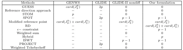
(c) To propose a general algorithm for solving an MOP, it is necessary to convert the MOP problem to a general scalarized problem with per-haps some additional constraints. It is obvious that the number of constraints added to the general scalarized problem has a major effect on the computational time. In Table 1 (for nondifferentiable MOPs) we compare the number of constraints added to the suggested gen-eral formulation (3) with those added to some gengen-eral formulations as GLIDE [21], GLIDE-II [28] and GENWS [32].
Table 1: Number of additional constraints in each formulation (in nondiffer-entiable case)
Methods GENWS GLIDE GLIDE-II nondiff Our formulation
GUESS card(Jk
2) 2p 0 0
Reference direction approach − − 0 0
STOM p − 0 0
SPOT − 2p p−1 p−1
Modified reference point card(Jk
2) +card(J
k
3) − card(J
k
3) card(J
k
3)
RD − − − card(Jk
2) +card(J
k
3)
ϵ−constraint − − − p−1
Weighted sum − − 0 0
Hybrid − − − p
ISWT − − p−1 p−1
PROJECT − 2p 0 0
Weighted Tchebycheff − − 0 0
(d) One of the most important theoretical advantages of the proposed gen-eral formulations is that, Theorem 5 enables us to provide results con-cerning proper efficiency. Unboundedness of the trade-offs means, prac-tically, ignoring at least one of the objective functions when the DM wants to improve another objective function, which is not satisfactory to the DM. Since properly efficient solutions have bounded trade-offs, the DM can improve some unacceptable objective functions with no concern.
(e) All the provided theorems where established without convexity assump-tions. In fact, the main MOP can be convex or nonconvex.
7 A numerical example
An interactive algorithm for solving multiobjective optimization problems ... 95 problem, has two conflicting objective functions. We should minimize the volume of the truss (f1), and its joint displacement (f2), subject to given physical restrictions on the feasible cross-sectional areasx1, x2, x3,andx4 of the four bars. The stress on the truss structure is caused by several forces of magnitudeF,and 2F.The lengthLof each bar and the elasticity constantsE
andσof the materials involved are modelled as constants. The mathematical model of this example is as follows:
Minimize
{
f1(x) =L(2x1+
√
2x2+
√
2x3+x4),
f2(x) = F L
E ( 2 x1 +2 √ 2 x2 −2 √ 2 x3 + 1 x4 ) } s.t. F
σ ≤x1≤ 3F
σ ,
√
2(Fσ)≤x2≤ 3σF,
√
2(F
σ)≤x3≤ 3F
σ , F
σ ≤x4≤ 3F
σ ,
where, the constant parameters are chosen as F = 10 kN, E = 2 × 10⁵ kN/cm2, L= 200cmandσ= 10kN/cm2.
The ideal and nadir values for objective functions of this problem are obtained as yI = (yI
1, yI2) = (1400,−5.7191×10⁻⁴) and yN = (yN1, y2N) = (3.4971×103,0.0406). Now, based on the GIA, at first, we should find an initial solution. To this end, the ϵ−constraint scalarizing problem (13) is used, which can be obtained from the proposed formulations by parameters and index sets given in Subsection 4.7,withl= 2 andϵ1= 1800.By solving the obtained problem, we find (1.3906,1.9963,1.4142,1.3957) for variables, and (1800,0.0157) for objective functions. As it can be seen, the values of the objective functions are between ideal and nadir values. Let ˆx1 = (1.3906,1.9963,1.4142,1.3957) andf(ˆx1) = (1800,0.0157) are shown to DM. Suppose, the DM wishes to express his/her preference information as the reference pointy¯1 = (¯y1
1,y¯21) = (1600,0.01). Based on this preference given by DM, one of the reference point based scalarizing problems can be selected. Here, we set parameters in our formulation, such that the GUESS scalariz-ing problem is obtained, and by solvscalariz-ing it, (1.4613,2.0666,1.4142,1.4613) is obtained for variables and (1861.3,0.0142) is attained for the objective func-tion values. At this iterafunc-tion, the volume of the truss has increased and its joint displacement has slightly decreased. Now, assume that the DM wants to change the type of his/her preference information. According to Step 5 of the GIA, set ˆx2 = (1.4613,2.0666,1.4142,1.4613), f(ˆx2) = (1861.3,0.0142) andk= 2.Now, Step 3 is executed.
96 M. Ghaznavi, M. Ilati and E. Khorram the RD scalarizing problem is used with α = 0.5. By solving the problem, (1.1876,1.6796,1.4142,1.1876) is obtained for variables and (1587.6,0.0221) is attained for the objective functions. Assume that the DM wants to provide new preferences by selecting weights for the objective functions. To this end, let ˆx3 = (1.1876,1.6796,1.4142,1.1876), f(ˆx3) = (1587.6,0.0221), and
k = 3. Then, Step 4 is executed by (w3
1, w32) = ( 3 4,
1
4) as weights given by the DM. By solving the weighted sum problem (14), (1,1.4142,1.4142,1) is obtained for variables and (1400,0.03) is obtained for the objective values. As it can be seen, the volume of the truss is in its ideal value, and this satisfies the DM. It is important to point out that by Theorem 5, the obtained objective vector is a properly nondominated point.
8 Conclusions
In this article, we suggested a general scalarizing formulation to obtain a global interactive algorithm for multiobjective optimization problems. We proposed the formulation in two versions; one of them for differentiable and the other for nondifferentiable MOPs. By selecting suitable values for pa-rameters, we proved that optimal solutions of the suggested general scalar-izing problem are (weakly, properly) efficient solutions for the main mul-tiobjective problem. Moreover, it was shown that many scalarizing prob-lems used in different interactive methods as GUESS, reference direction approach, Step, STOM, SPOT, modified reference point, and RD methods can be obtained from the proposed general formulation, by selecting suitable transformations. Some of the popular scalarizing problems such as, weighted sum,ϵ−constraint, and hybrid problems derived from our general scalarizing problem. In addition, we proposed a general interactive algorithm. In the proposed algorithm, the DM could express his/her preference information in six different ways, and based on the kind of information given by the DM, a suitable scalarizing problem, by selecting appropriate values for parame-ters and index sets in the general formulation, was selected. Finally, by a numerical example we illustrated that how the proposed general interactive algorithm can be used.
However, for the future investigation, developing a software based on the suggested general interactive algorithm can be worthwhile. Also, proposing a general interactive procedure for approximate efficient solutions of an MOP can be worth studying. To this end, studying three recently published papers by Ghaznavi-ghosoni1 and Khorram [10], Ghaznavi-ghosoni et al. [11] and Ghaznavi [12] is recommended.
An interactive algorithm for solving multiobjective optimization problems ... 97
Acknowledgments:
The authors would like to express their heartfelt thanks to the editors and anonymous referees for their useful suggestions which improved the quality of the paper.
References
1. Benayoun, R., Montgolfier, J., Tergny, J. and Laritchev, O. Linear pro-gramming with multiple objective functions: Step method (STEM), Math-ematical Programming 1(3) (1971) 366-375.
2. Buchanan, J.T. A naive approach for solving MCDM problems: the GUESS method, Journal of the Operational Research Society 48 (1997) 202-206.
3. Chankong, V. and Haimes, Y.Y.The interactive surrogate worth trade-off (ISWT) method for multiobjective decision-making, in: S. Zionts (Eds.), Multiple Criteria Problem Solving, Berlin: Springer, 1978, pp. 42-67. 4. Ehrgott, M. Multicriteria Optimization, Springer, Berlin, 2005.
5. Engau, A. and Wiecek, M.M. Generating ε−efficient solutions in mul-tiobjective programming, European Journal of Operational Research 177 (2007) 1566-1579.
6. Eschenauer, H.A., Osyczka, A. and Schafer, E. Interactive multicriteria optimization in design process, in: Eschenauer, H., Koski, J., Osyczka A., (Eds.), Multicriteria Design Optimization Procedures and Applications, Berlin: Springer, 1990, pp. 71-114.
7. Gardiner, L. and Steuer, R.E. Unified interactive multiple objective pro-gramming, European Journal of Operational Research 74(3) (1994) 391-406.
8. Gardiner, L. and Steuer, R.E. Unified interactive multiple objective pro-gramming: an open architecture for accommodating new procedures, Jour-nal of the OperatioJour-nal Research Society 45(12) (1994) 1456-1466.
9. Geoffrion, A. Proper efficiency and the theory of vector maximization, Journal of Mathematical Analysis and Applications 22 (1968) 618-630. 10. Ghaznavi-ghosoni, B.A. and Khorram, E. On approximating
98 M. Ghaznavi, M. Ilati and E. Khorram 11. Ghaznavi-ghosoni, B.A., Khorram, E. and Soleimani-damaneh, M.
Scalarization for characterization of approximate strong/weak/proper effi-ciency in multiobjective optimization, Optimization, 62 (6) (2013) 703-720. 12. Ghaznavi, M. Optimality conditions via scalarization for approximate
quasi efficiency in multiobjective optimization, Filomat, accepted. 13. Hosseinzadeh Lotfi, F., Jahanshahloo, G.R., Ebrahimnejad, A.,
Soltani-far, M. and Mansourzadeh, S.M.Target setting in the general combined-oriented CCR model using an interactive MOLP method, Journal of Com-putational and Applied Mathematics 234(1) (2010) 1-9.
14. Jahn, J. Vector Optimization: Theory, Applications, and Extensions, Springer-Verlag, Berlin, Germany, 2004.
15. Kaliszewski, I. A modified weighted Tchebycheff metric for multiple ob-jective programming, Computers and Operations Research 14 (1987) 315-323.
16. Kaliszewski, I. A theorem on nonconvex functions and its application to vector optimization, European Journal of Operational Research 80 (1995) 439–449.
17. Kaliszewski, I. Using trade-off information in decision making algo-rithms, Computers and Operations Research 27 (2000) 161–182.
18. Kaliszewski, I. and Michalowski, W. Efficient solutions and bounds on tradeoffs, Journal of Optimization Theory and Applications 94 (1997) 381-394.
19. Kaliszewski, I., Miroforidis, J. and Podkopaev, D. Interactive multiple criteria decision making based on preference driven evolutionary multiob-jective optimization with controllable accuracy, European Journal of Op-erational Research 216 (2012) 188-199.
20. Korhonen, P. Reference direction approach to multiple objective linear programming: Historical overview, in: Karwan, M. H., Spronk,J., Wal-lenius, J., (Eds.), Essays in Decision Making: A Volume in Honour of Stanley Zionts, Springer-Verlag, Berlin, Heidelberg, 1997, pp. 74-92. 21. Luque, M., Ruiz, F. and Miettinen, K.Global formulation for interactive
multiobjective optimization, OR Spectrum 33(1) (2011) 27–48.
22. Luque, M., Yang, J.B. and Wong, B.Y.H.PROJECT method for multiob-jective optimization based on the gradient projection and reference point, IEEE Transactions on Systems, Man and Cybernetics-Part A: Systems and Humans 39(4) (2009) 864-879.
An interactive algorithm for solving multiobjective optimization problems ... 99 24. Nakayama, H. and Sawaragi, Y. Satisficing trade-off method for multi-objective programming, in: M. Grauer, A.P. Wierzbick (Eds.), Interactive Decision Analysis, Berlin: Springer, 1984, pp. 113-122.
25. Narula, S.C., Kirilov, L. and Vassilev, V.Reference direction approach for solving multiple objective nonlinear programming problems, IEEE Trans-actions on Systems, Man, and Cybernetics 24 (1994) 804-806.
26. Park, K.S. and Shin, D.E. Interactive multiobjective optimization ap-proach to the inputoutput design of opening new branches, European Jour-nal of OperatioJour-nal Research 220 (2012) 530-538.
27. Romero, C.Extended lexicographic goal programming: a unified approach, Omega 29 (2001) 63-71.
28. Ruiz, F., Luque, M. and Miettinen, K.Improving the computational ef-ficiency in a global formulation (GLIDE) for interactive multiobjective optimization, Annals of Operations Research 197(1) (2012) 47-70. 29. Sakawa, M. Interactive multiobjective decision making by the sequential
proxy optimization technique: SPOT, European Journal of Operational Research 9 (4) (1982) 386-396.
30. Taras, S. and Woinaroschy, A.An interactive multiobjective optimization framework for sustainable design of bioprocesses, Computers & Chemical Engineering 43 (2012) 10-22.
31. Vassilev, V., Narula, S.C. and Gouljashki, V.G.An interactive reference direction algorithm for solving multiobjective convex nonlinear integer pro-gramming problems, International Transactions in Operational Research 8 (4) (2001) 367-380.
ﯽﻣﻮﻤﻋ
۲مﺮﺧ ﻞﯿﻋﺎﻤﺳا و۲ﯽﺗﻼﯾا ﺪﻤﺤﻣ ،۱یﻮﻧﺰﻏ دادﺮﻬﻣ
یدﺮﺑرﺎﮐ ﯽﺿﺎﯾر هوﺮﮔ ،ﯽﺿﺎﯾر مﻮﻠﻋ هﺪﮑﺸﻧاد ،دوﺮﻫﺎﺷ هﺎﮕﺸﻧاد۱ ﺮﺗﻮﯿﭙﻣﺎﮐ مﻮﻠﻋ و ﯽﺿﺎﯾر هﺪﮑﺸﻧاد ،ﺮﯿﺒﮐﺮﯿﻣا ﯽﺘﻌﻨﺻ هﺎﮕﺸﻧاد۲
١٣٩۴ ﺮﻬﻣ ٢٩ ﻪﻟﺎﻘﻣ شﺮﯾﺬﭘ ،١٣٩۴ ﺮﯿﺗ ١٣ هﺪﺷ حﻼﺻا ﻪﻟﺎﻘﻣ ﺖﻓﺎﯾرد ،١٣٩٣ ﺪﻨﻔﺳا ٣ ﻪﻟﺎﻘﻣ ﺖﻓﺎﯾرد
ار هﺪﻧﺮﯿﮔ ﻢﯿﻤﺼﺗ ﻪﮐ ﯽﻣﻮﻤﻋ ﯽﻠﻣﺎﻌﺗ یﺎﻫﻢﺘﯾرﻮﮕﻟا ﻪﯾارا ﻪﺑ زﺎﯿﻧ ،دﻮﺟﻮﻣ ﯽﻠﻣﺎﻌﺗ یﺎﻫشور عﻮﻨﺗ : هﺪﯿﮑﭼ
.ﺪﻫدﯽﻣ نﺎﺸﻧ ار ﺪﻨﮐ بﺎﺨﺘﻧا ار ﺖﺳا وا ﺢﯿﺟﺮﺗ درﻮﻣ ﻪﮐ ار ﺐﺳﺎﻨﻣ شور ﻦﯾﺪﻨﭼ ﻪﻧادازآ ﻪﮐ ﺪﻧزﺎﺳﯽﻣ ردﺎﻗ دﺎﻬﻨﺸﯿﭘ ﻪﻓﺪﻫ ﺪﻨﭼ یﺰﯾرﻪﻣﺎﻧﺮﺑ ﻞﺋﺎﺴﻣ یاﺮﺑ ﯽﻣﻮﻤﻋ یزﺎﺳﺮﻟﺎﮑﺳا ﻪﻠﺌﺴﻣ ﮏﯾ ،ﻪﻟﺎﻘﻣ ﻦﯾا رد ،رﻮﻈﻨﻣ ﻦﯾا یاﺮﺑ یارﺎﮐ و (ﻒﯿﻌﺿ) ارﺎﮐ یﺎﻫ باﻮﺟ و هﺪﺷ ﯽﻓﺮﻌﻣ یزﺎﺳﺮﻟﺎﮑﺳا ﻪﻠﺌﺴﻣ ﻪﻨﯿﻬﺑ یﺎﻫ باﻮﺟ ﻦﯿﺑ ﻪﻄﺑار .ﻢﯿﻫدﯽﻣ ،ﺐﺳﺎﻨﻣ یﺎﻫﻞﯾﺪﺒﺗ بﺎﺨﺘﻧا ﺎﺑ ﻪﮐ ﻢﯿﻫدﯽﻣ نﺎﺸﻧ .دﻮﺷﯽﻣ ﯽﺳرﺮﺑ ﯽﻠﺻا ﻪﻓﺪﻫ ﺪﻨﭼ یزﺎﺳﻪﻨﯿﻬﺑ ﻪﻠﺌﺴﻣ هﺮﺳ هﺪﺷ دﺎﻬﻨﺸﯿﭘ لﻮﻣﺮﻓ زا ﺪﻨﻧاﻮﺗﯽﻣ ﻒﻠﺘﺨﻣ ﯽﻠﻣﺎﻌﺗ یﺎﻫشور رد ﻪﺘﻓر رﺎﮐ ﻪﺑ یزﺎﺳﺮﻟﺎﮑﺳا ﻞﺋﺎﺴﻣ زا ﯽﺧﺮﺑ ﻪﮐ ﻢﯿﻫدﯽﻣ دﺎﻬﻨﺸﯿﭘ ﯽﻣﻮﻤﻋ ﯽﻠﻣﺎﻌﺗ ﻢﺘﯾرﻮﮕﻟا ﮏﯾ ،هﺪﺷ دﺎﻬﻨﺸﯿﭘ یزﺎﺳﺮﻟﺎﮑﺳا ﻪﻠﺌﺴﻣ سﺎﺳا ﺮﺑ .ﺪﻨﯾآ ﺖﺳﺪﺑ ﺮﻫ رد تﺎﺤﯿﺟﺮﺗ رد ﺮﯿﯿﻐﺗ ﺖﯿﻠﺑﺎﻗ ﺎﺑ و ﻒﻠﺘﺨﻣ شور ﺶﺷ ﺎﺑ ار ﺶﺗﺎﺤﯿﺟﺮﺗ ﺪﻨﮐ ﯽﻣ ردﺎﻗ ار هﺪﻧﺮﯿﮔ ﻢﯿﻤﺼﺗ ﻢﺘﯾرﻮﮕﻟا ندﻮﺑ یدﺮﺑرﺎﮐ ﺮﮕﻧﺎﯿﺑ ﻪﮐ یدﺪﻋ لﺎﺜﻣ ﮏﯾ ،مﺎﺠﻧاﺮﺳ .ﺪﻨﮐ ﺺﺨﺸﻣ ﻢﺘﯾرﻮﮕﻟا یﺎﻫراﺮﮑﺗ لﻮﻃ رد نﺎﻣز .ددﺮﮔﯽﻣ ﻪﯾارا ﺖﺳا