Max Planck Institute for Demographic Research Konrad-Zuse Str. 1, D-18057 Rostock·GERMANY www.demographic-research.org
DEMOGRAPHIC RESEARCH
VOLUME 25, ARTICLE 2, PAGES 39-102
PUBLISHED 5 JULY 2011
http://www.demographic-research.org/Volumes/Vol25/2/ DOI: 10.4054/DemRes.2011.25.2
Research Article
More on the cohort-component model of
population projection in the context of HIV/
AIDS: A Leslie matrix representation
and new estimates
Jason R. Thomas
Samuel J. Clark
c
°2011 Jason R. Thomas & Samuel J. Clark.
2 CCMPP 42
2.1 The HIV incidence trend 46
2.2 Additional HIV-related force of mortality 48
2.3 Matrix notation for HIV-enabled CCMPP 52
3 Parameter estimation 56
3.1 Data types 56
3.2 Likelihoods 59
3.2.1 HIV test results in a general-population sample 60
3.2.2 HIV test results in an ANC-patient sample 61
3.2.3 HIV test results in all or a sample of births from HIV-positive mothers 62 3.2.4 HIV test results during a follow-up of an HIV-negative sample 63 3.2.5 Survival during a follow-up of HIV+ individuals 63
3.3 Parameter estimation 64
4 Results 65
4.1 Modeling survival for the infected population 69 4.2 An application to a rural South African population 79
5 Discussion 86
6 Acknowledgements 88
More on the cohort-component model of population projection in the
context of HIV/AIDS: A Leslie matrix representation
and new estimates
Jason R. Thomas1
Samuel J. Clark2
Abstract
This article presents an extension of the cohort-component model of population projection (CCMPP) first formulated by Heuveline (2003) that is capable of modeling a population affected by HIV. Heuveline proposes a maximum likelihood approach to estimate the age profile of HIV incidence that produced the HIV epidemics in East Africa during the 1990s. We extend this work by developing the Leslie matrix representation of the CCMPP, which greatly facilitates the implementation of the model for parameter estimation and projection. The Leslie matrix also contains information about the stable tendencies of the corresponding population, such as the stable age distribution and time to stability. Another contribution of this work is that we update the sources of data used to estimate the parameters, and use these data to estimate a modified version of the CCMPP that includes (estimated) parameters governing the survival experience of the infected population. A further application of the model to a small population with high HIV prevalence in rural South Africa is presented as an additional demonstration. This work lays the foundation for development of more robust and flexible Bayesian estimation methods that will greatly enhance the utility of this and similar models.
1Center for Demography of Health and Aging, University of Wisconsin-Madison.
E-mail: [email protected].
2Department of Sociology, University of Washington. Institute of Behavioral Science (IBS), University of
1. Introduction
The cohort-component model of population projection (CCMPP) is perhapsthe iconic method in demography, see for example Bowley (1924); Cannan (1895); Whelpton (1936); Leslie (1945); Pritchett (1891); Pearl and Reed (1920); Dorn (1950). This classic method moves incrementally forward in time a population defined by age according to a specified life table and set of age-specific fertility rates, taking into account net migration at each age. In its basic form it is straightforward and easy to implement, which has allowed it to become one of the essential tools used by governments and planning organizations to help them understand the likely future size and composition of a population, and how that may change under different assumptions or as a result of interventions of various types.
Fundamentally the CCMPP relates the age structure of a population to fertility, mor-tality, and migration, with the current age structure being the result of fertility, mortality and migration at each age in the past. Most commonly a future age structure of the popula-tion is ‘predicted’ given a time series of age-specific fertility, mortality, and net migrapopula-tion. The model can also be used toestimatetrends in a subset of the four components given the others, and it is a use of this type that occupies us here.
The HIV epidemic affecting Africa and other parts of the developing world poses significant challenges to demographers concerned with either measuring the current state of an affected population or predicting its future. Because HIV affects both fertility and mortality in important ways (Sewankambo et al. 1994; Nunn et al. 1997; Carpenter et al. 1997; Gray et al. 1998; ˙Zaba and Gregson 1998; Todd et al. 1997; Wachter, Knodel, and Van Landingham 2002; Hunter et al. 2003; Terceira et al. 2003; Lewis et al. 2004; Timaeus and Jasseh 2004; Ford and Hosegood 2005; Garenne et al. 2007; Gregson et al. 2007; Kahn et al. 2007; Nyirenda et al. 2007; ˙Zaba et al. 2007; Clark et al. 2008), it is not possible to understand the dynamics of a population affected by HIV without specifically taking into account these effects. Further complicating this situation, data describing underlying fertility and mortality unaffected by HIV are scarce and often of poor quality, especially for most populations with high HIV prevalence.
These challenges are addressed in an interesting and useful way in a model developed by Heuveline (2003). Heuveline created a multi-state version of the standard CCMPP model (Day 1996; United Nations 2004) that further classifies the population by time since infection with HIV, and uses a set of age-specific incidence parameters to ‘in-fect’ HIV negative people and transition them to the first (shortest duration) HIV positive group. This version of the model also includes additional parameters to govern the links between HIV status and fertility. Heuveline used data describing HIV status and sur-vival (mortality) from East African countries to estimate these model parameters, using maximum likelihood techniques.
multi-state, HIV-enabled CCMPP in the following ways. Since the original publication of this model in 2003, more data have become available on HIV prevalence and the survival of those infected. Perhaps the most notable source of more recent data is the Demo-graphic and Health Surveys (DHS) program (and the associated AIDS Indicator Surveys – AIS) which have collected information on age-specific HIV prevalence from nationally-representative population-based surveys. We augment the data compiled by Heuveline (2003), taken from sources in East Africa, with over 100,000 observations on HIV preva-lence provided by the DHS data in the same region.3 We estimate the model parameters
using the augmented data and compare these new estimates to those obtained by using only the data compiled by Heuveline, as well as to the estimates obtained by using only the more recent data compiled by us. Adding more recent data to the analysis will provide more information about the later stages of the HIV epidemic, and the comparisons across the data compilations will show how sensitive the estimates are to the data being used (particularly with respect to the date when the data were collected).
Relative to the original data used, there is more recent information on the survival of those infected with HIV (e.g. ˙Zaba et al. 2007; Crampin et al. 2002; Urassa et al. 2001; Sewankambo et al. 2000) which motivates an extension of the CCMPP model. Previous work with the HIV-enabled CCMPP uses a fixed survival schedule for the infected popu-lation to estimate the model parameters (see the next section for more details). While it is possible to specify (a priori) a reasonable survival schedule for HIV-positive individuals, it is preferable to let data inform the model, so that the estimates and projections are not influenced by problems with the assumed mortality experience. In this paper we extend the CCMPP to include additional parameters that govern the survival of the infected pop-ulation, and estimate these parameters using new data gathered from the literature. It is worth noting that the estimated age pattern of HIV incidence may be sensitive to the life table used for the infected population, because the incidence parameters are estimated us-ing data on HIV prevalence, which is a function of both incidence and survival. In other words, an observed level of HIV prevalence can arise from different combinations of in-cidence and survival rates. Given this point, we discuss differences in the estimated age patterns of HIV incidence between the original specification of the model and the version in which survival for the infected population is estimated. A final point that motivates our extension of the model is that the expansion of antiretroviral treatment programs will affect the survival prospects of the infected population. The modeling techniques car-ried out here are easily adaptable to a population with significant access to antiretroviral treatment, which makes CCMPP an additional tool to study the future effects of these treatment programs.
3The list of countries from which DHS data are used consists of Ethiopia, Kenya, Malawi, Rwanda, Tanzania,
The final contribution of our work is to shift the geographic focus from eastern Africa to South Africa, where the HIV epidemic has reached even higher levels (UNAIDS 2008). Data on age-specific HIV prevalence from a population living in a rural area of the KwaZulu-Natal province of South Africa (Welz et al. 2007) is used to estimate the CCMPP parameters, and these estimates are compared to those obtained from the data collected in eastern Africa. Different parameterizations of the model are also explored along with the long term implications for the age structure.
The subsequent sections of this paper are organized as follows. A detailed introduc-tion of Heuveline’s multi-state, HIV-enabled CCMPP is provided in the next secintroduc-tion, with the Leslie matrix representation of the model. This is followed by a description of the data and a brief discussion of the maximum likelihood estimation used in the analysis. The focus then shifts to the results obtained from using the new data and the modeling of the survival of the infected population. Finally, we apply the CCMPP to a rural population in South Africa and conclude with a discussion section.
2. CCMPP
Heuveline (2003) extends the standard CCMPP to accommodate a population categorized by duration of infection with HIV using five ‘HIV duration’ groups. There are four HIV+ duration groups (0-4 years, 5-9 years, 10-14 years, and 15+ years) as well as an HIV– group. In this section we present Heuveline’s multi-state CCMPP for a population with 17 age groups (0-4, 5-9, . . . , 80+) in each of the five HIV duration groups. The model is introduced with a series of equations representing the transition from one group/time pe-riod to the next. While the model can be applied to both men and women, the description presented here only includes the details for women.
Begin by dividing the population into age groups wherea= 1,2, . . . ,17correspond to age groups 0-4, 5-9,. . ., 80+. Denote membership in the HIV duration groups byd, withd = 1,2, . . . ,5 corresponding to HIV–, HIV+ for 0-4 years,. . . ,HIV+ for more than 15 years. Time is indexed bytnoting that the duration betweentandt+ 1is equal to the width of a standard age interval, i.e. 5 years. Letna,d,tbe the number of women in age groupaand duration groupdat timet. For1< a <17, we have:
na+1,1,t+1 = na,1,tsa,1,t(1−ia,t) (1)
na+1,2,t+1 = na,1,tsa,1,tia,tsa,2 (2)
to the same underlying base survivorship ratio as the HIV– group, in addition to this extra survivorship ratio that accounts for the increased mortality associated with different durations of infection. The parameteria,tis the fraction of women in age groupawho become infected with HIV over the projection interval. To allow for the heterogeneity of HIV epidemics across populations, this parameter is decomposed as:
ia,k,t= 1−exp{−Γt,t0·H·ja,k} (4)
wherek denotes sex and Γt, t0 is a parametric curve used to model the time trend in
the HIV epidemic from the start time t0. The actual values for Γt, t0 are presented in
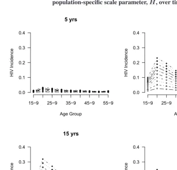
Table 1 (see the next section for more details). The parameterHis a population-specific scale parameter that captures the overall magnitude of the epidemic. The parameterja,k is an age- and sex-specific scaling factor for incidence that represents the multiplicative difference in HIV incidence between age groupaand a reference age group, which is held constant at a value of 1.0 in order to make the model identifiable. Following Heuveline, we set the reference age group females aged 25-29, i.e.j5,f emale= 1.0.
For a given age profile of incidence (a specific set of values forja), Figure 1 demon-strates how the different values forH simply scale the incidence profile. Each panel in this figure corresponds to a different time in the epidemic, with incidence, whose overall scale is determined by the values ofΓ. Within each panel, each line corresponds to a value of the population-specific scale parameterH ranging from 0.1 to 1.0.
The projection equations are slightly different for the youngest and oldest age groups. The oldest (open-ended) age group is incremented by two sources, those 75-79 and 80+ in the previous time period. Thus fora= 17we have:
n17,1,t+1 = n16,1,ts16,1,t(1−i16,t)
+ n17,1,ts17,1,t(1−i17,t) (5)
n17,2,t+1 = n16,1,ts16,1,ti16,ts16,2
+ n17,1,ts17,1,ti17,ts17,2 (6)
n17,d,t+1 = n16,d−1,ts16,1,ts16,d
+ n17,d−1,ts17,1,ts17,d for 2< d <5 (7)
n17,5,t+1 = n16,4,ts16,1,ts16,5+n17,4,ts17,1,ts17,5
Figure 1: Age-specific HIV incidence rates,ia,t, for different values of the population-specific scale parameter,H, over time
0.0 0.1 0.2 0.3 0.4 5 yrs Age Group H IV I n c id e n c e
15 9 25 9 35 9 45 9 55 9
0.0 0.1 0.2 0.3 0.4 10 yrs Age Group H IV I n c id e n c e
15 9 25 9 35 9 45 9 55 9
0.0 0.1 0.2 0.3 0.4 15 yrs Age Group H IV I n c id e n c e
15 9 25 9 35 9 45 9 55 9
0.0 0.1 0.2 0.3 0.4 20 yrs Age Group H IV I n c id e n c e
15 9 25 9 35 9 45 9 55 9
projection interval, taking into account the fact that HIV+ women who have been infected for different durations will, to varying degrees, be less likely to have children. To cap-ture the relationship between fertility and HIV status, Heuveline defined three additional parameters. First, consider the number of HIV– births:
n1,1,t+1 = s0,1,t 1
1 +SRB ×
¡Xβ
a=α
fa,1,t
na,1,t+p−a−1,1,tna−1,1,t
2
+
5
X
d= 2
β X
a=α fa,d,t−
na,d,t+pa−1,d−1,tna−1,d−1,t
2
¢
. (9)
In Equation 9 above,SRBis the sex ratio at birth, thefa,1,t’s are simply the age-specific fertility rates for HIV– women, and the lower and upper bounds of the childbearing age range areα andβ. Fertility among HIV+ women introduces the following parameters
f−
a,d,t = fa,1,tea gd(1−v) (10)
for1 < d. The superscript infa,d,t− designates HIV– births (i.e. d= 1) to women who are HIV+. The parametervd is the probability that an HIV+ woman in duration group
d will give birth to an HIV+ child, the vertical transmission rate. The parameterea captures the higher level of sexual activity and resulting fertility among HIV+ women age 15-19 who have been infected for 0-4 years (d = 2). In other words we expect
ea=4>1whileea6=4are constrained to be 1.0. The parametergdrepresents thefertility
impairmentexperienced by women in duration groupd, a number that becomes smaller as the time since infection increases, reflecting increasing fertility impairment with time since infection. The corresponding equations for HIV+ births are:
n1,2,t+1 = s0,1,t 1
1 +SRB
5
X
d= 2 β
X
a=α
f+ a,d,t
na,d,t+pa−1,d−1,tna−1,d−1,t
2 (11)
f+
a,d,t = fa,1,tea gdv. (12)
Finally, we define the factors used to approximate the average number of women at the beginning and end of the period,p−
a,1,t andpa,d,t:
p−
a,1,t = sa,1,t(1−ia,t) (13)
pa,1,t = sa,1,tia,tsa,2 (14)
2.1 The HIV incidence trend
Recall that age-specific incidence in CCMPP is modeled as follows:
ia,k,t= 1−exp{−Γt,t0H ja,k}
whereia,k,t is the fraction of individuals agea who will become infected over the pro-jection interval. Γt, t0 represents the shape of the incidence trend from the start of the
epidemic in yeart0 to the projection periodt. This incidence trend is shifted up or down byH, an overall scale parameter for the epidemic. Finally, ja,k is the incidence ratio comparing those of ageaand sexkto women age 25-29. The details of the incidence trendΓt, t0are described in this section, along with several other possible specifications.
The incidence trendΓt, t0 used by Heuveline (2003) is borrowed fromEpiModel,
a computer program developed by the World Health Organization to make short-term projections of adult AIDS cases (Chin and Lwanga 1991) (the precursor of EPP, UNAIDS’ estimation and projection package software used to estimate the prevalence of HIV (Ghys et al. 2004)), and is based on the gamma family of distributions:
g(t) = t
α−1e−x/β
(α−1)!βα, for t≥0, α >0β >0. (16) Theαparameter is typically referred to as the shape parameter since it affects how peaked or flat the density is; asα increases the density appears more flat or uniform. The scale parameterβis associated with how diffuse or spread out the density is; asβ increases the density spreads out.
Before discussing the calculations made by Heuveline (2003) it is helpful to discuss a particular property of the gamma distribution. The mode, or the the value for which the the function reaches its maximum, is equal to(α−1)β. This quantity has a nice interpretation in that it is the number of years after the start of the epidemict0when the epidemic peaks. For example, if the shape parameters is 5 and the scale parameter is 3, then the epidemic peaks 12 years after it began.4
4Chin and Lwanga (1991) report that settingα= 5results in “the best empirical ‘fit’ to the reported AIDS-case
This is precisely the density used by Heuveline (2003) to calculate the five-year inci-dence rates (i.e.α= 5, β= 3). The actual rates are calculated by integrating the gamma density over the appropriate five-year span, i.e.:
Γx,t0 =
Z x
(x−5)
t5−1e−x/3
(5−1)!35dt for5≥x≤20, (17)
Γ20+,t0 = 5×
Z 21
20
t5−1e−x/3
(5−1)!35dt. (18)
The five-year incidence rate for twenty years after the start date is different because the decline in the gamma density for values greater than 20 is too rapid to represent an actual decline in incidence. The values used to estimate the CCMPP parameters are presented in Table 1. We are aware that this is relatively crude, and it would be preferable to model this trend using time series techniques with attention given to the uncertainty around the trend, especially at time points far into the future. That is among the improvements that currently occupy us.
Table 1: Five-year incidence rates calculated from the gamma density and an exponential curve
Time Period Γt,t0 Et,t0
0 - 5 years 0.028 0.063
6 - 10 years 0.216 0.191
11 - 15 years 0.316 0.323
16 - 20 years 0.235 0.457
20+ yearsa 0.163 0.540
Notes: aFor the gamma model it is assumed that the HIV incidence rate will level off at the rate equal to the integral
of the gamma density from 20 and 21 multiplied by five. For the exponential model it is assumed that the HIV incidence rate will level off at a rate equal to5∗(h(t= 21)−h(t= 20)). See the text for the definition ofh(t).
We will now discuss two other possible specifications for the trend in HIV incidence. The first is an exponential curve that models a continual increase in HIV over time. While this may not be realistic in the long run, it does provide an upper bound for the trend. A reasonable lower bound is a constant rate of new infections (i.e. no change) over time. Since the second specification is simply a constant5 we will focus our attention on the
exponential model.
The exponential curve used to model the trend in HIV incidence takes the following functional form:
h(t) = eβt
β −t for t= 1,2,3, . . .; and β >0. (19)
The five-year HIV incidence rates are calculated by differencingh(t) (at lag one) and summing over the five year period of interest:
Et, t0 =
5
X
j=1
h(t)−h(t−1) (20)
Heuveline (2003) chooses a value ofβ = 0.005 to obtain the five-year HIV incidence rates based on the exponential model, shown in Table 1. Finally, similar to the gamma model described above, the incidence rate after twenty years takes a different form. For the exponential curve,E20+,t0 = 5×(h(t= 21)−h(t= 20)).
2.2 Additional HIV-related force of mortality
In the HIV-enabled CCMPP individuals infected with HIV (d > 1) experience an addi-tional force of mortality that is not experienced by those in the HIV– state (d= 1). This mortality differential can be seen in the following projection equations
na+1,d= 2,t+1 = na,d= 1,tsa,d= 1,tia,tsa,d= 2 (21)
na+1,d >2,t+1 = na,d−1,tsa,d= 1,tsa,d >2 (22) wheresa,d >1 < 1; survival in the HIV+ states is reduced compared to the HIV– state. Recall that the vital rates in CCMPP are treated as fixed parameters and need to be set by the user.
group (40+ years).6 Similar results are reported in an updated analysis of these Ugandan
data by Van der Paal et al. (2007), and in other cohort studies carried out in sub-Saharan Africa (Lutalo et al. 2007; Isingo et al. 2007; Murray et al. 2007).
Given the evidence from the epidemiological literature, Heuveline (2003) specifies the survival rates for HIV+ individuals as a function of age at infection. This dependence comes through in the choice of a particular survival schedule, defined by the median number of years lived after infection. The schedules include median survival times of 3, 8, 10, and 12 years, which is consistent with the empirical evidence from sub-Saharan Africa (Newell et al. 2004; Marston et al. 2005; Morgan et al. 2002; Van der Paal et al. 2007; Lutalo et al. 2007; Peters et al. 2007; Isingo et al. 2007). Children who are infected perinatally follow the 3 year schedule, while the oldest age groups follow the 8-year schedule. Before describing the age dependence in greater detail, it is helpful to take a slight digression and define some more notation.
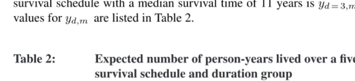
Heuveline (2003) defines these survival schedules with reference to the projection interval (i.e. five years). Letyd,m be the expected number of years lived by an individual in duration groupdfollowing survival schedulem, wherem= 3,8,11,12. For example, the average number of years lived by a person infected 5-9 years ago who is following the survival schedule with a median survival time of 11 years isyd= 3,m= 11 = 3.375. The values foryd,m are listed in Table 2.
Table 2: Expected number of person-years lived over a five-year interval by survival schedule and duration group
Survival Schedule
Duration Group 3 8 11 12
0 to 0-4 (d=2) 2.7750 4.7100 4.8000 4.8310
0-4 to 5-9 (d=3) 0.4250 2.4300 3.3750 3.6000
5-9 to 10-4 (d=4) 0.0000 0.8600 2.0000 2.4125
10-4 to 15-9 (d=5) 0.0000 0.3150 1.0000 1.5375
Now we are in a position to define sa,d >1. Let us begin with those who have been infected for 0-4 years (d= 2). Children born and infected (perinatally) during the projec-tion interval are exposed to:
sa=1,d=2=yd=2,m=3
5 . (23)
6In this same study, the median time from seroconversion to AIDS is 9.4 years, IQR: 5.5 – 10.1 years. The
The HIV-related survival ratios for the next two age groups are defined to be 1.0 because persons between the of ages 5 and 9 are not able to be infected given our current assump-tions about incidence. Recall that the age-specific incidence rates are zero for the first three age groups.7 For those who are ages 15-19, 25-34, or above age 45, the additional
force of mortality caused by HIV takes a form similar to the equation just above:
sa=4,d=2 = yd=2,m5 =12 = 0.9662 (24)
s8≥a≥6,d=2 = yd=2,m5 =11 = 0.9600 (25)
sa≥10,d=2 = yd=25,m=8 = 0.9420. (26) Note how survival declines as age increases before leveling off at age 45 and above. For the age groups not already mentioned, the survival parameters are calculated by taking the average over two adjacent survival schedules:
sa=5,d=2 = yd=2,m=11+2yd=2,m=12 = 0.9631 (27)
sa=9,d=2 = yd=2,m=8+2yd=2,m=11 = 0.9510. (28) We now turn our attention to the third duration group, individuals who have been infected for 5-9 years. For this group, we start with those ages 5-9:
sa=2,d=3 = yd=3,m=3
yd=2,m=3
. (29)
The corresponding parameters for the older age groups take a similar form. The expected number of years lived for the third duration group is divided by the expected number of years lived by the second duration group (for a given survival schedule). The dependence on age ford= 3takes the same form as for the previous duration group, only that the age groups are incremented by one. The actual equations are:
sa=5,d=3 = yd=3,m=3
yd=2,m=3 (30)
sa=6,d=3 = yd=3,m=12+yd=3,m=11
yd=2,m=12+yd=2,m=11 (31)
s9≥a≥7,d=3 = yd=3,m=11
yd=2,m=11
(32)
sa=10,d=3 =
yd=3,m=11+yd=3,m=8
yd=2,m=11+yd=2,m=8 (33)
sa≥11,d=3 =
yd=3,m=8
yd=2,m=8. (34)
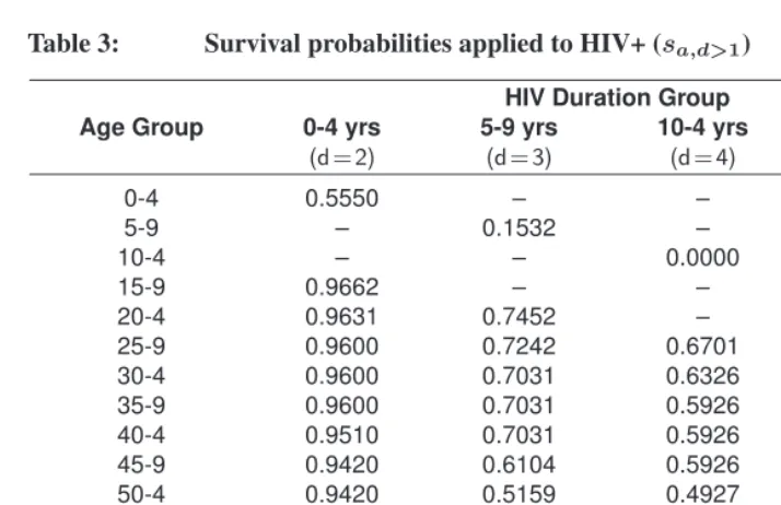
The pattern continues for the fourth and fifth duration groups. All of the parameters for the additional force of mortality due to HIV are listed in Table 3.
Table 3: Survival probabilities applied to HIV+ (sa,d>1)
HIV Duration Group
Age Group 0-4 yrs 5-9 yrs 10-4 yrs 15+ yrs
(d=2) (d=3) (d=4) (d=5)
0-4 0.5550 – – –
5-9 – 0.1532 – –
10-4 – – 0.0000 –
15-9 0.9662 – – 0.0000
20-4 0.9631 0.7452 – –
25-9 0.9600 0.7242 0.6701 –
30-4 0.9600 0.7031 0.6326 0.6373
35-9 0.9600 0.7031 0.5926 0.5751
40-4 0.9510 0.7031 0.5926 0.5000
45-9 0.9420 0.6104 0.5926 0.5000
50-4 0.9420 0.5159 0.4927 0.5000
55-9 0.9420 0.5159 0.3539 0.4598
60-4 0.9420 0.5159 0.3539 0.3663
65-9 0.9420 0.5159 0.3539 0.3663
70-5 0.9420 0.5159 0.3539 0.3663
75-9 0.9420 0.5159 0.3539 0.3663
80+ 0.9420 0.5159 0.3539 0.3663
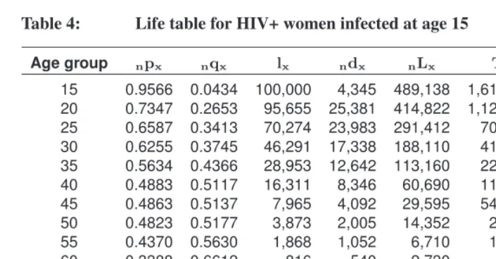
Life tables can also be constructed using the survival rates presented in Table 3, where cohorts defined by age at infection are exposed to the survival rates aligned along the diagonal cells of the table. For example children infected by their mothers will never reach age 15 years because the survival probability is zero for those infected at birth and between the ages of 10 and 14. The mortality experienced by the cohort of women infected at age 15 is summarized in the life table presented in Table 4.
Table 4: Life table for HIV+ women infected at age 15
Age group npx nqx lx ndx nLx Tx
0 e
15 0.9566 0.0434 100,000 4,345 489,138 1,612,020 16.1202
20 0.7347 0.2653 95,655 25,381 414,822 1,122,882 11.7389
25 0.6587 0.3413 70,274 23,983 291,412 708,060 10.0757
30 0.6255 0.3745 46,291 17,338 188,110 416,648 9.0006
35 0.5634 0.4366 28,953 12,642 113,160 228,538 7.8934
40 0.4883 0.5117 16,311 8,346 60,690 115,378 7.0736
45 0.4863 0.5137 7,965 4,092 29,595 546,880 6.8660
50 0.4823 0.5177 3,873 2,005 14,352 25,093 6.4789
55 0.4370 0.5630 1,868 1,052 6,710 10,741 5.7498
60 0.3388 0.6612 816 540 2,730 4,031 4.9395
65 0.3220 0.6780 276 187 912 1,301 4.7125
70 0.2940 0.7060 89 63 288 389 4.3669
75 0.2500 0.7500 26 20 80 101 3.8713
80 0.1586 0.8414 6 6 21 21 3.4425
2.3 Matrix notation for HIV-enabled CCMPP
These equations for the multi-state, HIV-enabled CCMPP can be conveniently expressed in matrix notation. For a population with 17 age groups and five HIV duration groups, the population at timetis represented by an85×1column vector
nt =
n1,1,t
n2,1,t .. .
n17,1,t .. .
n1,4,t
n2,4,t .. .
n17,4,t
The correspondingLesliematrix is:
At=
B1,1 B1,2 B1,3 B1,4 B1,5 B2,1 B2,2 B2,3 B2,4 B2,5 0 B3,2 0 0 0 0 0 B4,3 0 0 0 0 0 B5,4 B5,5
(36)
whereBi,jis a17×17sub-matrix that models how groupjat timetcontributes to group
iat timet+1. Note thatB3,1is a zero matrix since women who are HIV– at timetcannot give birth to children who have been HIV positive for ten years byt+ 1(i.e. five years into the future). Similar reasoning applies for the other zero matrices.
The calculations involvingB1,j produce the projection for the number of HIV– births (i.e. n1,1,t+1) contributed by duration groupj. Similarly, B2,j projects the number of HIV positive births contributed by duration group j > 1. B1,1 andB2,1 are a little different in that they project each age group to the next oldest age groupandfrom one HIV duration group to the next. Let us first considerB1,1:
B1,1=
b−
1,1,t b−2,1,t · · · b−17,1,t
p−1,1,t 0 · · · 0
0 p−2,1,t . .. ...
0 0 . .. 0
..
. ... . .. . .. 0 0
0 0 · · · 0 p−
16,1,t p−17,1,t
. (37)
Recall that the number in the first age group at timet+ 1is equal to the number of births summed across the fecund age groups. Letb−a,d,t be the factor needed to calculate the number of HIV– births to mothers in age groupaat timetand in duration groupd:
b−a,1,t = s0,1,t 1
1 +SRB f
−
a,1,t
1 +p−a−1,1,tna−1,1,t na,1,t
2 . (38)
In our application of the multi-state, HIV-enabled CCMPP, fertility only occurs among women aged 15-49 (i.e. α= 4, β= 10). Consequentlyb−
a <4,1,t = b−a >10,1,t = 0. In the equation above the factorna−1,1,t
of giving birth. If the count in the denominatorna,1,tis ever zero the entire ratio is simply replaced by zero. This issue arises when dealing with the fertility of the HIV+ groups. The same procedure is used in the analogous HIV+ equations if they involve dividing by zero.
B1,dford >1projects forward HIV– births contributed by duration groupdand can be written as:
B1,d=
b−1,d,t b−2,d,t b−3,d,t · · · b−17,d,t
0 · · · 0
.. . . .. 0 0 (39) where
b−a,d,t = s0,1,t 1
1 +SRB f
−
a,d,t
1 +pa−1,d−1,t(na−na,d,t1,d−1,t)
2 (40)
ford > 1. TheB2,d’s determine the number of people infected with HIV for less than five years at timet+ 1, contributed by those in duration groupdat timet. For the first duration group we have:
B2,1=
b+
1,1,t b+2,1,t · · · b+17,1,t
p1,1,t 0 · · · 0
0 p2,1,t . .. ...
0 0 . .. 0
..
. ... . .. . .. 0 0
0 0 · · · 0 p16,1,t p17,1,t
B2,dford > 1projects forward the number of HIV+ births contributed by duration groupd. It can be written as:
B2,d=
b+1,d,t b+2,d,t b+3,d,t · · · b+17,d,t
0 · · · 0
.. . . .. 0 0 (42) where
b+a,d,t = s0,1,ts0,1,t 1
1 +SRB f
+ a,d,t
1 +pa−1,d−1,t(na−na,d,t1,d−1,t)
2 . (43)
The remaining non-zero sub-matrices – B3,2,B4,3,B5,4andB5,5 – project people forward in both age and time, and consequently the only non-zero elements occur along the sub-diagonal:
Bi,j=
0 0 · · · 0
p1,d=j,t 0 · · · ...
0 p2,d=j,t . ..
0 0 . .. 0
..
. ... . .. . .. 0 0
0 0 · · · 0 p16,d=j,t p17,d=j,t
. (44)
3. Parameter estimation
The CCMPP projections are used to estimate thirty-three of the model parameters. As mentioned earlier, the vital rates, the initial population counts and the HIV survival sched-ules are all fixed. The 33 parameters we estimate are:
• v: vertical transmission parameter that is constrained to be between 0 and 1; al-though the model is described as having a vertical transmission rate for each dura-tion group, there are not enough data to estimate separate parameters. (1 parameter) • ea: fertility selection parameter that is constrained to be equal to 1 for all groups except women aged 15-19 in the first HIV duration group, for whom we expect the value to be greater than 1. (1 parameter)
• gd: fertility impairment parameter for women in duration groupd, ford= 2,3,4; the fertility impairment parameter ford= 5 is constrained such thatgd=5=gd=4, and the values for all duration groups are constrained to be between 0 and 1. (3 parameters)
• ja,k: relative incidence ratio parameter that is constrained to be equal to 1 for women age 25-29 and non-negative for all other groups; values are estimated for women (k= 1) age15−19,20−24,30−34,35−39, . . . ,55−59and for men (k= 2) in the age groups between 15-59 (i.e. 8 and 9 age-specific parameters for women and men, respectively). (17 parameters)
• Hh: scale parameters for the trend in HIV incidence for populationh. (11 parame-ters)
For a given set of parameter values, we obtain a set of not necessarily unique age- and sex-specific counts. These model outputs are used to calculate predicted values for the observed data. For example the ratio of the projected number of HIV+ women age 20-25 over the total number of women projected in that age group, is used to predict the observed HIV prevalence for women in that age group. Several types of observed data, such as HIV prevalence, are used to estimate the values of the parameters that are most likely.
In this section we discuss this topic in greater detail. The first focus is on the types of data used in the analysis. We then shift to the likelihoods specific to each type of data. Finally we turn to the techniques used to estimate the parameters, namely maximum likelihood (ML) estimation.
3.1 Data types
col-lected from antenatal clinics (ANCs), demographic surveillance sites, hospitals and gen-eral surveys. Both rural and urban areas are included, and the years of data collection range from 1989 to 1998. The data are classified into the following five categories (see Table 1, Heuveline 2003):
1. HIV test results in a general-population sample (10 data sets)
2. HIV test results in an ANC-patient sample (3 data sets)
3. HIV test results in all or a sample of births from HIV+ mothers (3 data sets)
4. HIV test results during a follow-up of an HIV– sample (3 data sets)
5. Survival during a follow-up of HIV+ individuals (3 data sets)
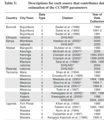
In addition to the data compiled by Heuveline, several new sources are also included in the analysis carried out here. All of the data sources are listed in Table 5, with the sources unique to the current analysis appearing in the shaded rows.
Although we have updated the information used to estimate the CCMPP parameters, we are unable to exploit many of the published results in the literature because those data are not broken down by age. For example, vertical transmission and the subsequent survival of infected infants has been the focus of a great deal of research (e.g. Simonon et al. 1994; Miotti et al. 1999; Spira et al. 1999; Nicoll et al. 2000; De Cock et al. 2000; Nduati et al. 2000; Mandelbrot et al. 2002; Petra Study Team 2002; Jackson et al. 2003; Read and Breastfeeding and HIV International Transmission Study Group 2004; Newell et al. 2004; Zijenah et al. 2004; Marston et al. 2005; Brahmbhatt et al. 2006; Kagaayi et al. 2008). While much has been learned from these studies, the published information is not stratified by the age of the mother, which would allow us to estimate the rate of vertical transmission by HIV duration groups. Without this level of detail, the CCMPP estimate of the vertical transmission rate is simply an average across all the estimates weighted by sample size. If future studies in this area tabulate the data by age of the mother it would greatly benefit modeling efforts.8 Similarly, many of the results concerning the
survival of infected individual (e.g. Van der Paal et al. 2007; Lutalo et al. 2007; Smith et al. 2007; Peters et al. 2007; Isingo et al. 2007; Murray et al. 2007), as well as HIV incidence and prevalence rates (e.g. Urassa et al. 2006; ˙Zaba et al. 2000; Wambura et al. 2007) are not reported by age.9 Small sample sizes may be a limiting factor, but we
encourage future studiesto report age-specific resultswhenever possible so that others can utilize the patterns observed along this critical dimension.
8The median survival time of children infected with HIV is around two years (Newell et al. 2004). Thus,
the CCMPP model, which classifies the population intofive-yearage groups, can contribute very little to this question.
9Age-specific results are available for other geographic regions (e.g. Nyirenda et al. 2007), but we restrict our
Table 5: Descriptions for each source that contributes data used in the estimation of the CCMPP parameters
Country City/Town Data
Citation
Year of Start Urban/
Type Data Year of Rural
Collection Epidemic
Burundi Bujumbura 1 Saidel et al. (1996) 1990 1973 Urban
Bujumbura 2 Sokal et al. (1993) 1991-2 1973 Urban
Bujumbura 4 Saidel et al. (1996) 1991 1973 Urban
Ethiopia national 1 DHS/AISa 2005 1980 National
Kenya Mombasa 1 Hawken et al. (2002)a 2000 1974 Urban
national 1 DHS/AISa 2003 1980 National
Malawi Mangochi 2 Slutsker et al. (1994) 1990 1975 Urban
Karonga 1 McGrath et al. (2007)a 2005 1975 Rural
Karonga 2 Crampin et al. (2008)a 1994-2001 1975 Rural
Karonga 5 Crampin et al. (2002)a 1998-2000 1975 Rural
Blantyre 2 Taha et al. (1998)a 1990, 1995 1975 Urban
national 1 DHS/AISa 2004 1980 National
Rwanda national 1 DHS/AISa 2005 1976 National
Tanzania Mara 1 Shao et al. (1994) 1990 1975 Urban
Mwanza 1 Grosskurth et al. (1995) 1992 1975 Rural
Mwanza 1 Mwaluko et al. (2003)a 1994, 1999 1975 Rural
Mwanza 4 Boerma et al. (1999)a 1994-7 1975 Rural
Mwanza 5 Urassa et al. (2001)a 1994-8 1975 Rural
Mwanza 5 Todd et al. (1997) 1994 1975 Rural
Kagera 1 Kwesigabo et al. (2005)a 1987, 1996 1975 Urban
Kagera 1 Kwesigabo et al. (2005)a 1996 1975 Rural
national 1 DHS/AISa 2004, 2007 1980 National
Uganda Fort Portal 1 Kilian et al. (1999) 1995 1975 Urban
Gulu 2 Fabiani et al. (2001) 1993, 1997 1975 Rural
Masaka 1 Nunn et al. (1994) 1989 1975 Rural
Masaka 2 Carpenter et al. (1997) 1990 1975 Rural
Masaka 4 Kengeya-Kayondo et al. (1996) 1990-4 1975 Rural
Masaka 4 Shafer et al. (2008)a 1995-2005 1975 Rural
Masaka 5 Nunn et al. (1997) 1990 1975 Rural
Rakai 1 Wawer et al. (1991) 1989-91 1980 Rural
Rakai 4 Wawer et al. (1994) 1990 1980 Rural
Rakai 1 Serwadda et al. (1992) 1989-91 1980 Rural
Rakai 2 Gray et al. (1998) 1995 1980 Rural
Rakai 5 Sewankambo et al. (1994) 1980 1990 Rural
Rakai 5 Sewankambo et al. (2000)a 1994-8 1980 Rural
Nsambya & Jinja
Table 5: (Continued)
Country City/Town
Data Citation Year of Start Urban/
Type Data Year of Rural
Collection Epidemic
Uganda Nsambya,
Jinja, & Rubaga
2 Asiimwe-Okiror et al. (1997)a 1995 1975 Urban
national 1 DHS/AISa 2004 1980 National
Zambia Chelston 1 Fylkesnes et al. (1998) 1995 1975 Urban
Kapiri Mposhi 1 Fylkesnes et al. (1998) 1996 1980 Rural
Lusaka 3 Hira et al. (1989) 1987 1975 Urban
national 1 DHS/AISa 2002,2007 1976 National
Zimbabwe Mutasa 1 Gregson and Garnett (2000) 1998 1977 Rural
Manicaland 1 Gregson et al. (2002)a 2000 1976 Rural
national 1 DHS/AISa 2006 1980 National
Data types: (1) HIV test results in a general-population sample; (2) HIV test results in an ANC-patient sample;
(3) HIV test results in all or a sample of births from HIV+ mothers; (4) HIV test results during a follow-up of an HIV– sample; (5) Survival during a follow-up of HIV+ individuals
Notes: The data sources that are unique to the current analysis appear in the shaded rows.
aNew sources of data not included in the compilation used by Heuveline (2003). DHS/AIS refers to the
Demographic and Health Survey program and the AIDS Indicator Surveys.
It should be noted that the CCMPP also requires vital rates for the uninfected popula-tion and an initial age distribupopula-tion. These model inputs are taken from the United Napopula-tions global population estimates (United Nations 1999) and model life tables (United Nations 1982).
3.2 Likelihoods
Each category of data provides the pieces needed for a proportion which leads to the use of the binomial distribution in the likelihood specification. The binomial likelihood can be written as:
L=Y µN
x
Before discussing the finer details of how the CCMPP outputs are used in the like-lihood, it is important to cover two points. First, we need to temporally match up the CCMPP projections with the observed data. The start year for the model is the year when widespread transmission of HIV began,t0. The population is then projected forward to the year when the data were collected. For example if widespread transmission in a coun-try began in 1980 and the observed data are from 2000, then we can take the projected counts 20 years from the start time and compare these to the observed data. Given that the projections are in five year increments, it is sometimes necessary to take the average across two projection periods to match the year of data collection. Estimates of when widespread HIV transmission began are taken from a report by the United Nations (1998, Table 1).
Second, the data come from populations at twenty-six different locations.10 At a
given location there can also be several different types of data. For example data from the population living in Mwanza, Tanzania, include both HIV prevalence from a general population and survival information for those who are HIV+. As a result there is a separate likelihood for the 51 combinations of location, year, and data type retrieved from the literature. These are indicated usinghfor the population (and location) andcfor the type or category of data. Finally, the data consist of sex- and age-specific information so the likelihoods may also be indexed by these characteristics as well.
3.2.1 HIV test results in a general-population sample
Various studies have collected data on sex- and age-specific HIV prevalence in a sample from the general population. The age groups range from 15-19 to 55-59. This type of data, labeled ‘1’ (c = 1), usually includes the number of people tested and the percent who tested positive for HIV by sex and age. The likelihood, however, requires a count of individuals who are HIV+, so we calculate this quantity from the data and round it to the nearest integer. LetNa,k,t,h,c= 1 denote the total number of individuals in age groupa of sexk at timetat locationhand letxa,k,t,h,c= 1 be the number in this group who tested positive.
na,d,t,h the projected counts from CCMPP are used to predict sex- and age-specific prevalence for a given location as follows:
πa,k,t,h,c=1=
P5
d=2na,d,t,h
P5
d=1na,d,t,h
, (46)
where the sum is taken across HIV duration groups. Having chosen the projection period that matches up with the year the data were observed, we can use πa,k,t,h,c= 1 in the binomial likelihood. A final note is that the observed data may be reported by age groups that do not match those of our projections. In this case weighted sums of the projected counts can be used to estimate HIV prevalence. For example if observed prevalence is reported for individuals age 17-25, then predicted prevalence can be calculated as:
πage=(17−25),k,t,h,c=1=
P5
d=2(na=4,d,t,h×0.6 +na=5,d,t,h)
P5
d=1(na=4,d,t,h×0.6 +na=5,d,t,h)
. (47)
This issue arises with the other data types as well.
3.2.2 HIV test results in an ANC-patient sample
Seven of the data sets used in this analysis provide age-specific information on HIV preva-lence for female attendees of ANCs, typically from age 15 to 49. This type of data, indexed byc = 2, takes a form similar to the observed prevalence from a general pop-ulation, except that they only refer to women. Both the total number of women tested
Na,k= 1,t,h,c= 2and the age-specific prevalence are reported. The data are included in the binomial likelihood as counts, so we calculate the number of women who tested positive
xa,k=t,hrounded to the nearest integer.
The predicted prevalence for the ANC attendees is calculated differently than for the general population. Recall that there are two primary assumptions of CCMPP concerning the fertility of HIV+ women. The first is that HIV+ women age 15-19 have higher fertility which is captured by the fertility selection parameterea= 4. Second, fertility is expected to decline as time since infection increases, modelled by the fertility impairment param-etersgd >1. Since the HIV+ women observed in the data are pregnant, these parameters are included in the calculation of predicted prevalence. The formula is:
πa,k= 1,t,h,c= 2=
P5
d=2na,d,k=1,t,h×ea×gd
na,d,k= 1,t,h+
P5
d=2na,d,k= 1,t,h×ea×gd
where the sum is taken over the duration groups. Having chosen the projection period that matches up with the year the data were observed, we can useπa,k= 1,t,h,c= 2 in the binomial likelihood.
3.2.3 HIV test results in all or a sample of births from HIV-positive mothers
Heuveline (2003) found three data sets consisting of information on the fertility of HIV+ women. However one of these sources, Hira et al. (1989), differs from the others in that it provides information on whether or not an HIV+ mother infected her child. Data from the other two sources, Carpenter et al. (1997) and Gray et al. (1998), consist of the number of children born to both HIV+ and HIV– women, by age group. The likelihoods for the latter two sources are nearly identical to those in the data categoryc= 2, HIV test results in an ANC sample. The only difference is that the observed counts (i.e. the data) refer to the total number of children born to female ANC attendees in a specific age group, and the number of children born to HIV+ attendees. The probability that a child is born to an infected mother is calculated in exactly the same way asπa,k= 1,t,h,c= 2. Given this similarity the data reported by Carpenter et al. (1997) and Gray et al. (1998) are classified here asc= 2.
Data that take the form of Hira et al. (1989) will also be indicated byc = 3. The corresponding counts used in the likelihood refer to the total number of children born to infected mothers in age groupo,No,t,h,c= 3, and the number of these children who are infected by their mothersxo,d= 2,t,h,c= 3. The predicted rate of vertical transmission using the model outputs is calculated as:
πo,t,h,c= 3=
P5
dP=2na,k=1,d,t,h×fa,d= 1,t,h×ea×gd×vd 5
d=2na,k=1,d,t,h×fa,d=1,t,h×ea×gd
, (49)
where the sum is taken over the duration groups.
3.2.4 HIV test results during a follow-up of an HIV-negative sample
Data on sex- and age-specific HIV incidence are also used to estimate CCMPP parame-ters. These data indexed byc= 4are typically reported in terms of the number of people who become infected and the total number of person-years lived while uninfected. For the binomial likelihood however, we need the counts of the initial population observed
Na,t,d= 1,t,h,c= 4 and the number who become infectedXa,t,d= 2,t,h,c= 4. Thus the ini-tial population size needs to be calculated from the observed data, and this calculation can be done as follows:
Initial Population= # Converted
1−exp
n
−T ×Person-Years# Converted
o (50)
whereT is the total number of years observed.11
The model outputs are then used to calculate the probability of becoming infected for men or women in a certain age group at a given location and time. That is:
πa,k,d= 1,t,h,c= 4=na,k,d=1,t,h×sa,k,d=1,t,h−na+1,k,d=1,t+1,h
na,k,d=1,t,h×sa,k,d=1,t,h (51) whereπa,k,d= 1,t,h,c= 4 is the proportion of HIV– women/men who become infected after five years. As discussed earlier, the period of observation for the data may not be equal to the projection interval of five years. If the observation period is only four years, then the quantity of interest is calculated as:
1−exp
½
4 5×log
µ
1− # Converted Initial Population
¶¾
. (52)
3.2.5 Survival during a follow-up of HIV+ individuals
The final category of data describes the survival (mortality) of HIV+ individuals. This category indexed byc= 5is similar to the previous one in that the data reported include the number of deaths observed among a cohort of HIV+ individuals of a particular age and sexXa,k,t,h,c= 5and the number of person-years observed for each group. As be-fore, the likelihoods require the initial population size for each groupNa,k,t,h,c= 5 (see Equation 50). These two inputsXa,k,t,h,c= 5 andNa,k,t,h,c= 5are the counts needed for
11In deriving this equation it is helpful to note that the number of person-years lived by a population of initial
the binomial likelihood with the corresponding proportion referring to the probability of death over a given period of time.
The procedure for calculating the probability of death from the model outputs is best described in two steps. First, we calculate the probabilities by age, sex, and duration group. This can be written as:
qa,k,d,t,h,c= 5 = 1−
µ
na+1,k,d+1,t+1,h
na,k,d,t,h
¶T
5
for d ≥ 2 (53)
whereT is the number of years over which the data were observed. Since the observed data do not contain information on duration group, we must calculate the weighted av-erage where the weights are the counts in each duration group. This second step is per-formed as follows:
πa,k,t,h,c= 5=
P5
d=2qa,k,d,t,h,c= 5×na,k,d,t,h
na,k,d,t,h
. (54)
This is the probability used in the binomial likelihood.
3.3 Parameter estimation
A maximum likelihood (ML) approach is used to estimate the most likely parameter val-ues (given the data and the model) and the uncertainty around those point estimates. Given the data from an individual site, the likelihood of a specific set of CCMPP parameter val-ues can be calculated using the binomial expressions described above. There are twenty-two likelihoods in the original data compilation and an additional twenty-nine likelihoods included in the analysis below. We follow Heuveline (2003) and combine these likeli-hoods by taking the product across all locations and data types, assuming independence. The set of parameter values that maximizes the combined likelihood is the ML point esti-mate.
4. Results
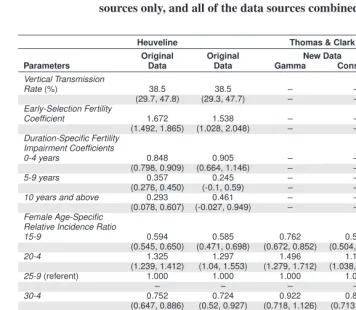
Five sets of ML estimates for the CCMPP parameters are presented in Table 6, with the 95% confidence intervals shown in parentheses. The first column of estimates (moving from left to right) contains the results published by Heuveline (2003) and the second col-umn lists our replication of his work using the same data. The point estimates for these two sets of results are generally consistent, as is seen with the vertical transmission rate. In both of the analyses it is estimated that 38.5% of children born to HIV+ mothers will be infected by their mothers, with the confidence intervals reaching from a low of around 30% to a high of nearly 48%. This result is well in line with previous estimates of verti-cal transmission in sub-Saharan Africa that range from 25% to 45% (Nicoll et al. 2000; Marston et al. 2005).12 Both sets of results also suggest that infected women 15 to 19
years old have fertility that is considerably higher than HIV– women in the same age group. The multiplicative factor by which fertility is higher among infected women is equal to the early-selection fertility coefficient times the fertility impairment coefficient for women infected less than five years. These factors are 1.42 for Heuveline’s estimates and 1.39 for our replication of his analysis using the same data. The fertility of women infected for five or more years is estimated by Heuveline to be lower than that of un-infected women or those un-infected for less than five years. Our results are consistent in that the fertility of women who have been infected for 5 to 9 years is likely to be at least 40% lower than uninfected women (i.e. the upper bound of the 95% confidence inter-val is 0.60). However, the large amount of uncertainty around the fertility impairment coefficient for women who have been infected for 10 or more years makes it difficult to draw conclusions about the fertility experience of these women. Finally, our estimated age patterns of HIV incidence, for both women and men, are similar to those reported by Heuveline (2003). Among women the risk of infection is highest for those 20 to 24 years old, then the relative incidence ratios decline with age. There is a similar pattern for men, but the estimated risk of infection peaks at an older age group, those 25 to 29 years old. Although our estimate of the relative incidence ratio for men 15 to 19 years old is higher than that of Heuveline and our 95% confidence intervals tend to be wider,13 we feel that
our results are similar enough to Heuveline’s to justify using our implementation of the model to analyze the new data.14
12These estimates are higher than the 20% reported by Newell et al. (2004) from an analysis of data pooled
across sub-Saharan Africa, but the infection status of 17% of the children was undetermined.
13It is worth noting that some of our 95% confidence intervals include negative values, which is troubling given
that zero is the natural lower bound for the parameters. The same is true for the upper bound, namely 1.00, of the duration-specific fertility impairment coefficient for women infected for 0 to 4 years (5 to 9 years) when using gamma trend with the new data (all of the data) to estimate the parameters.
14For a given set of model inputs, our population projections match exactly those made by Heuveline. This
Table 6: Maximum likelihood estimates of the CCMPP parameters for the original data sources compiled by Heuveline (2003), the new data sources only, and all of the data sources combined
Heuveline Thomas & Clark
Original Original New Data All
Parameters Data Data Gamma Constant Data
Vertical Transmission
Rate(%) 38.5 38.5 – – 38.5
(29.7, 47.8) (29.3, 47.7) – – (29.4, 47.6)
Early-Selection Fertility
Coefficient 1.672 1.538 – – 1.954
(1.492, 1.865) (1.028, 2.048) – – (1.578, 2.330)
Duration-Specific Fertility Impairment Coefficients
0-4 years 0.848 0.905 – – 0.749
(0.798, 0.909) (0.664, 1.146) – – (0.576, 0.922)
5-9 years 0.357 0.245 – – 1.00
(0.276, 0.450) (-0.1, 0.59) – – (0.749, 1.251)
10 years and above 0.293 0.461 – – 0.433
(0.078, 0.607) (-0.027, 0.949) – – (0.138, 0.728)
Female Age-Specific Relative Incidence Ratio
15-9 0.594 0.585 0.762 0.564 0.849
(0.545, 0.650) (0.471, 0.698) (0.672, 0.852) (0.504, 0.623) (0.738, 0.960)
20-4 1.325 1.297 1.496 1.183 1.255
(1.239, 1.412) (1.04, 1.553) (1.279, 1.712) (1.038, 1.328) (1.499, 1.744)
25-9(referent) 1.000 1.000 1.000 1.000 1.000
– – – – –
30-4 0.752 0.724 0.922 0.877 0.975
(0.647, 0.886) (0.52, 0.927) (0.718, 1.126) (0.713, 1.041 (0.750, 1.200)
35-9 0.635 0.518 0.790 0.702 0.586
(0.482, 0.762) (0.32, 0.716) (0.554, 1.027) (0.553, 0.851) (0.403, 0.770)
40-4 0.551 0.577 0.686 0.551 0.807
(0.409, 0.795) (0.324, 0.83) (0.375, 0.996) (0.376, 0.725) (0.559, 1.055)
45-9 0.356 0.339 0.177 0.323 0.300
(0.159, 0.544) (0.085, 0.594) (-0.095, 0.450) (0.170, 0.476) (0.091, 0.509)
50-4 0.295 0.304 – – 0.112
(0.095, 0.679) (-0.021, 0.63) – – (-0.083, 0.307)
55-9 0.246 0.395 – – 0.176
(0.087, 0.627) (0.027, 0.764) – – (0.013, 0.338)
Table 6: (Continued)
Heuveline Thomas & Clark
Original Original New Data All
Parameters Data Data Gamma Constant Data
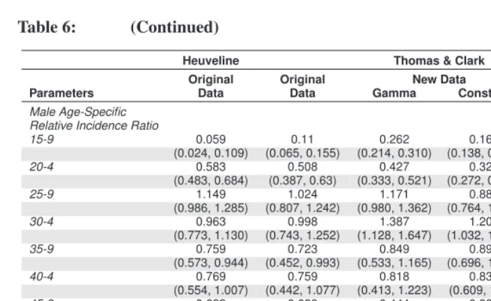
Male Age-Specific Relative Incidence Ratio
15-9 0.059 0.11 0.262 0.167 0.274
(0.024, 0.109) (0.065, 0.155) (0.214, 0.310) (0.138, 0.196) (0.226, 0.323)
20-4 0.583 0.508 0.427 0.329 0.466
(0.483, 0.684) (0.387, 0.63) (0.333, 0.521) (0.272, 0.385) (0.376, 0.556)
25-9 1.149 1.024 1.171 0.883 1.216
(0.986, 1.285) (0.807, 1.242) (0.980, 1.362) (0.764, 1.002) (1.033, 1.400)
30-4 0.963 0.998 1.387 1.201 1.383
(0.773, 1.130) (0.743, 1.252) (1.128, 1.647) (1.032, 1.370) (1.150, 1.617)
35-9 0.759 0.723 0.849 0.894 0.708
(0.573, 0.944) (0.452, 0.993) (0.533, 1.165) (0.696, 1.091) (0.485, 0.931)
40-4 0.769 0.759 0.818 0.835 1.088
(0.554, 1.007) (0.442, 1.077) (0.413, 1.223) (0.609, 1.062 (0.790, 1.385)
45-9 0.622 0.628 0.444 0.335 0.379
(0.409, 0.879) (0.297, 0.959) (0.145, 0.743) (0.137, 0.534) (0.130, 0.628)
50-4 0.417 0.288 0.519 0.458 0.483
(0.120, 0.773) (-0.093, 0.668) (0.145, 0.743) (0.249, 0.668) (0.194, 0.772)
55-9 0.168 0.219 0.526 0.466 0.189
(0.001, 0.445) (-0.114, 0.552) (0.081, 0.971) (0.189, 0.743) (-0.084, 0.462)
Log Likelihood -567 -580 -1799 -2121 -3444
Note: There are two sets of estimates based on the new data sources: one using the gamma trend for HIV incidence, and another using a constant trend. The 95% confidence intervals for each parameter are shown in parentheses.
makes it difficult to precisely identify the age at which the risk of infection peaks, the results suggest that men aged 30-34 experience the highest risk of infection. This is sligthly older than the peak age of infection for men estimated from the original data, the 25-29 year age group. This finding is particularly interesting given that the new data compilation consists of observations that are closer to the present, which may suggest that the age pattern of HIV incidence changes as the epidemic matures. Shafer et al. (2008) report a similar finding from a cohort study in Uganda. The results from the new data also suggest that the model based on the trend in HIV incidence derived from the gamma distribution fits the data better than a model with a constant trend in HIV incidence, as seen by comparing the log likelihoods for each model (gamma: -1790, vs. constant: -2121). Although the gamma trend fits these new data relatively well, the CCMPP estimates for more complicated models (presented in the next section) are much more unstable than those obtained from the specification of a constant incidence trend. Thus, a constant incidence trend is assumed for extensions of the CCMPP, and the corresponding results for the original model are presented here for the purpose of comparison.
4.1 Modeling survival for the infected population
One modeling assumption in the HIV-enabled CCMPP is that the lower survival rates associated with HIV/AIDS (captured by the parameterssa,dford≥2) are known. While it is possible to specify a realistic survival schedule for the infected population, a more appealing extension of the model is to estimate the additional force of mortality associated with HIV/AIDS. This approach also seems reasonable since there are more data available on the survival experiences of HIV+ cohorts that are not included in the original data compilation used by Heuveline (2003). Recall that the projected counts in the CCMPP are calculated as
na+1,1,t+1 = na,1,tsa,1,t(1−ia,t)
na+1,2,t+1 = na,1,tsa,1,tia,tsa,2
na+1,d,t+1 = na,d−1,tsa,1,tsa,d for d >2,
withsa,d≥2capturing the reduced survival prospects associated with HIV/AIDS for each duration group. Instead of treating these model inputs as fixed, we can estimate thesa,d≥2 in various ways. A parsimonious approach is to ignore the dependence on age at infec-tion15 and assume that survival is only a function of the duration of infection, which can
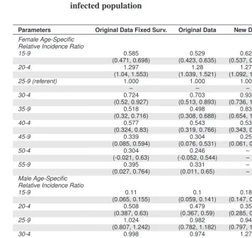
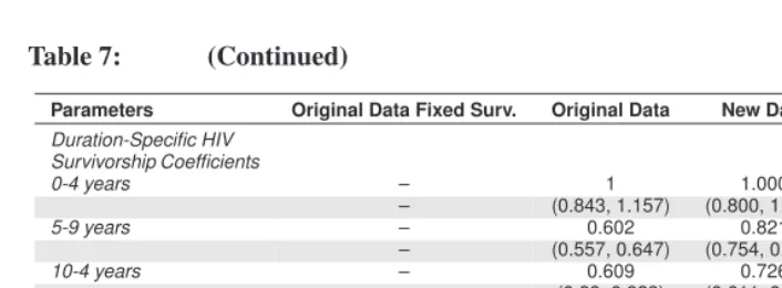
be expressed assd for d ≥ 2(dropping the subscript for age group). These four new model inputs (one for each HIV+ duration group) can be estimated along with the other CCMPP parameters estimated in the previous section. The results for this model are pre-sented in Table 7 along with estimates from the model with fixed survival, for the purpose of comparison. As with the previous results, estimates are shown for results obtained from using the original data compiled by Heuveline, the new data with the constant trend in HIV incidence, and all of the data sources combined.
15Heuveline (2003) specified the model so that expected survival time declines as the age at infection increases
Table 7: Maximum likelihood estimates for the modified CCMPP that includes duration-specific survivorship coefficients for the infected population
Parameters Original Data Fixed Surv. Original Data New Data All Data
Female Age-Specific Relative Incidence Ratio
15-9 0.585 0.529 0.621 0.837
(0.471, 0.698) (0.423, 0.635) (0.537, 0.705) (0.724, 0.950)
20-4 1.297 1.28 1.277 1.553
(1.04, 1.553) (1.039, 1.521) (1.092, 1.461) (1.316, 1.791)
25-9 (referent) 1.000 1.000 1.000 1.000
– – – –
30-4 0.724 0.703 0.930 0.891
(0.52, 0.927) (0.513, 0.893) (0.736, 1.123) (0.688, 1.093)
35-9 0.518 0.498 0.836 0.434
(0.32, 0.716) (0.308, 0.688) (0.654, 1.019) (0.266, 0.602)
40-4 0.577 0.543 0.534 0.822
(0.324, 0.83) (0.319, 0.766) (0.343, 0.725) (0.595, 1.048)
45-9 0.339 0.304 0.259 0.191
(0.085, 0.594) (0.076, 0.531) (0.061, 0.457) (-0.009, 0.392)
50-4 0.304 0.246 – 0.169
(-0.021, 0.63) (-0.052, 0.544) – (-0.058, 0.395)
55-9 0.395 0.331 – 0.171
(0.027, 0.764) (0.011, 0.65) – (-0.005, 0.346)
Male Age-Specific Relative Incidence Ratio
15-9 0.11 0.1 0.183 0.263
(0.065, 0.155) (0.059, 0.141) (0.147, 0.219) (0.216, 0.310)
20-4 0.508 0.479 0.354 0.493
(0.387, 0.63) (0.367, 0.59) (0.285, 0.422) (0.403, 0.583)
25-9 1.024 0.982 0.942 1.219
(0.807, 1.242) (0.782, 1.182) (0.797, 1.086) (1.046, 1.393)
30-4 0.998 0.974 1.277 1.283
(0.743, 1.252) (0.739, 1.209) (1.075, 1.478) (1.062, 1.504)
35-9 0.723 0.71 0.866 0.721
(0.452, 0.993) (0.461, 0.959) (0.642, 1.090) (0.510, 0.932)
40-4 0.759 0.705 0.842 0.726
(0.442, 1.077) (0.425, 0.986) (0.575, 1.110) (0.481, 0.971)
45-9 0.628 0.564 0.442 0.477
(0.297, 0.959) (0.27, 0.858) (0.189, 0.695) (0.238, 0.717)
50-4 0.288 0.197 0.360 0.204
(-0.093, 0.668) (-0.152, 0.545) (0.075, 0.646) (-0.064, 0.472)
55-9 0.219 0.183 0.331 0.108
Table 7: (Continued)
Parameters Original Data Fixed Surv. Original Data New Data All Data
Duration-Specific HIV Survivorship Coefficients
0-4 years – 1 1.000 1.000
– (0.843, 1.157) (0.800, 1.200) (0.922, 1.078)
5-9 years – 0.602 0.821 0.658
– (0.557, 0.647) (0.754, 0.889) (0.602, 0.714)
10-4 years – 0.609 0.726 0.611
– (0.29, 0.929) (0.611, 0.840) (0.451, 0.771)
15 years and above – 1 0.147 0.968
– (-2.887, 4.887) (0.043, 0.252) (0.612, 1.325)
Log Likelihood -580 -569 -2030 -3214
Notes: Results are presented for analyses obtained by using the original data compiled by Heuveline (2003), new data, and all of the data sources combined. The 95% confidence intervals for each parameter are shown in parentheses. Survival for the infected populations is equal to the product of these duration-specific coeffi-cients and the appropriate survivorship ratio applied to the uninfected population; see text for more details. (CCMPP parameters related to fertility are not shown.)