Volume 14 - Article 12 | Pages 237–266

in the population sciences published by the Max Planck Institute for Demographic Research Konrad-Zuse Str. 1, D-18057 Rostock · GERMANY www.demographic-research.org

DEMOGRAPHIC RESEARCH

VOLUME 14, ARTICLE 12, PAGES 237-266

PUBLISHED 28 MARCH 2006

http://www.demographic-research.org/Volumes/Vol14/12/ DOI: 10.4054/DemRes.2006.14.12

Research Article

The institutionalization and pace of fertility

in American stepfamilies

Jui-Chung Allen Li

2 Background 239

2.1 Fertility differentials by marital status 239

2.2 Stepfamily processes 239

2.3 Birth order and stepfamily fertility 240

2.4 Modeling the “catch up” effect of fertility 241

3 Method 245

3.1 Data and variables 245

3.2 Childbearing patterns: smoothed nonparametric fertility rates 246

4 Results 247

4.1 Descriptive statistics: parity definition of stepfamily status 247

4.2 Social norms of childbearing 248

4.3 Lifetime parity as fertility determinant and the

“institutionalization hypothesis”

251

4.4 The “pace” of fertility and the “institutionalization hypothesis” 253

4.5 Implications for completed cohort fertility 255

4.6 Speculations on the constant thirty-six month “pace” difference 256

5 Discussion 257

6 Acknowledgements 260

The institutionalization and pace of fertility

in American stepfamilies

Jui-Chung Allen Li 1

Abstract

This paper compares nonparametric fertility rates for American women in stepfamilies and intact families using data from the June 1995 Current Population Survey. Results show that childbearing behaviors in stepfamilies resemble those in intact families. Regardless of stepfamily status, timings and levels of fertility for second and third marital births are identical for all women at the same lifetime parity. Fertility patterns are also similar for all first marital births, with the exception of a constant three-year difference in the pace of fertility and a “fertility penalty” for stepfamily women. These findings are consistent with (1) the institutionalization hypothesis of stepfamily processes; (2) the hypothesis that lifetime parity is the primary determinant of female fertility; and (3) a speculation that women in stepfamilies attempt to catch up on lost fertility outside of marriage. These findings also imply that increasing prevalence of stepfamilies will not lead to increased completed fertility.

1. Introduction

Social changes in recent decades have profoundly altered the family as a reproductive institution (Ryder 1997). In the United States, the trend shifted from a majority of women born in the early twentieth century giving birth only within intact first marriages to increasing proportions of women in subsequent cohorts having diverse family trajectories involving divorce, remarriage, or nonmarital childbearing (Casper and Bianchi 2002; Wu and Li 2005). Stepfamilies have become increasingly a common context in which childbearing takes place due to the rising trends of marital disruption and out-of-wedlock births (Bumpass 1984a). Following Bumpass’s (1990) argument that demographic theories of fertility are “intrinsically about changes in the family as an institution” because childbearing “cannot be isolated from the institutional context in which it is embedded” (p. 483), the present study seeks to expand fertility research to incorporate the sociology of stepfamily, and to examine how childbearing behaviors in stepfamilies compare to childbearing behaviors in intact families.

A burgeoning body of fertility research has adopted stepfamily designs (e.g., Buber and Prskawetz 2000; Griffith, Koo, and Suchindran 1985; Henz 2002; Thomson 1997, 2004; Thomson and Li 2002; Thomson et al. 2002; Vikat, Thomson, and Hoem 1999; Vikat, Thomson, and Prskawetz 2004). These studies focus on identifying the effects of the subjective values of children on fertility. The stepfamily design provides the needed variation to identify the value of a child in demonstrating a couple’s commitment to a new cohabitation or marriage and the value of a child in conferring parental status. By contrast, there is no way to discern such values under the intact family design in which a first child in a cohabitation or marriage is also the first experience of becoming a parent for both partners. This line of research thus relies on the fertility variations by stepfamily types to address a fundamental question in demography: “what motivates an individual or couple to have children?” Despite its obvious importance, this question differs substantially from the focus of the more traditional demographic studies that document the differentials of fertility between intact families and stepfamilies.

2. Background

2.1 Fertility differentials by marital status

The traditional demographic approach to stepfamily fertility emphasizes the association between marital status and fertility. In hypothesizing that marital disruption reduces fertility by depriving a woman of exposure to the socially sanctioned, high-fertility institution of marriage, remarriage is seen to restore the woman’s reduced fertility by reinstating her married status. Empirical research has found that fertility is lower for women who have experienced a marital disruption (Cohen and Sweet 1974; Downing and Yaukey 1979; Lauriat 1969; Thornton 1978). The effect of remarriage on fertility is small but positive in narrowing the fertility differential between the divorced and the continuously married. For women with multiple remarriages, the small narrowing effect in each remarriage might cumulate across time so that they often end up with slightly higher completed fertility (Chen et al. 1974; Clarke et al. 1993; Cohen and Sweet 1974; Downing and Yaukey 1979; Ebanks et al. 1974; Thornton 1978). 2 Furthermore, two of the pioneer studies in this tradition connect the sociology of family processes with the demography of stepfamily fertility. Cohen and Sweet (1974) speculate marital discord might help explain the fertility differential between the divorced and continuously married. Thornton (1978) finds that fertility declined even in the two years before marital separation, which is consistent with Cohen and Sweet’s speculation on the negative effect of marital discord on childbearing.

2.2 Stepfamily processes

In his seminal work, Cherlin (1978) argues that stepfamilies suffer from a lack of social norms and well-defined social roles. Members of a stepfamily need to invent their own ways of social interaction, to redefine the family roles that are otherwise well established in the intact family, and to cope with potentially higher levels of economic and emotional strains. The “incomplete institutionalization” of stepfamilies manifests itself in their higher divorce rates compared with first marriages (e.g., McCarthy 1978), with the differential in divorce attributable to the presence of stepchildren (White and Booth 1985). Other scholars dispute the extent to which the selection effects hamper the “incomplete institutionalization” effects: stepfamilies may consist of a group of individuals who are, for instance, less religious, less inclined to stay in an unhappy

marriage, and more likely to marry the first time at younger ages (Booth and Edwards 1992; Castro Martin and Bumpass 1989; Furstenberg and Spanier 1984). Differences between stepfamilies and intact families, thus, may not indicate substantively meaningful differences in family processes yet reflect these selective characteristics. Furthermore, comparisons between stepfamilies and intact families often rely on cross-sectional data. But because stepfamilies are more likely to be observed at shorter durations than the intact families in a cross-sectional design, the differences between the two family types may be overstated in such studies.

Recent longitudinal studies have reported substantial similarities between intact families and stepfamilies, thereby supporting an alternative, “successfully-institutionalized-stepfamily” hypothesis (see Coleman et al. 2000 for a review). Stepfamilies do not suffer higher frequencies of marital conflict than intact families (MacDonald and DeMaris 1995); to the contrary, the differences in marital satisfaction between stepfamilies and intact families are found to be small and of little practical significance (Vemer et al. 1989). Patterns of family functioning in stepfamilies resemble those in intact families (Bogenscheider 1997; Peek et al. 1988; Waldren et al. 1990), especially at longer durations (O’Connor, Hetherington, and Reiss 1998; Vuchinich et al. 1991; Vuchinich et al. 1993). Clinicians observe that many stepfamilies gradually consolidate and stabilize (Papernow 1984, 1993), with the birth of a mutual child affording the much desired opportunity to hold families together (Bernstein 1989). As Coleman and colleagues (2000) cogently argue, “Even for those eventually disrupted remarriages, it is difficult to believe that they have made so many efforts to form a new family and never struggled to ‘institutionalize’ it and worked hard to ‘make it work’” (p. 1289). Efforts to adjudicate between the “incomplete institutionalization” and the “institutionalization” hypotheses are still inconclusive, but more and more studies rely on longitudinal data rather than a cross-sectional comparison to examine this question. No study has compared childbearing behaviors as an indicator of family processes.

2.3 Birth order and stepfamily fertility

Following the emphasis on birth order, this present paper identifies time dependences of parity-specific fertility rates, with a focus on two intertwined birth orders for the woman giving a birth: marital parity (Pm) and lifetime parity (Pl). Configurations of the two parities define a woman’s stepfamily status when she bears a child. Because a stepfamily is defined by the presence of stepchildren, when a woman bears a child in a stepfamily, her lifetime parity is greater than her marital parity (_Pl >_Pm

). But when a woman bears a child in an intact family, her two parities for this particular child are the same ( l m

P

P = ). Consider, for example, a woman whose first (lifetime) birth occurs unmarried at age twenty-one. After becoming married at age twenty-five, she gives her second (lifetime) birth in the marriage two years later. When she has another child, this child will be her third lifetime birth ( l=3

P ) and the

second birth in the same marriage (Pm =2). The last child is considered born into a stepfamily (_Pl >_Pm

) under the definition of this paper.

2.4 Modeling the “catch up” effect of fertility

Previous research also finds that younger children are more likely than their older counterparts to obtain a half sibling when their parents remarry (Buber and Prskawetz 2000; Bumpass 1984a; Griffith et al. 1985; Loomis and Landale 1994; Wineberg 1990, 1992). This implies that a large proportion of stepfamilies acquire a mutual child soon after remarriage, suggesting that there is motivation for women in stepfamilies to “catch up” on their lost reproductive time outside of marriage by having another child sooner in the new marriage.

Nevertheless, there exists no consensus over how to model the fertility “catch-up” phenomenon. Most studies have adopted a “relative-risks” approach to modeling fertility rates, specifying a proportional hazard model as follows:

...)r(t)=q(t)⋅exp(b₁x₁+b₂x₂+ (3),

or, equivalently, taking natural logarithm of both sides:

...logr(t)=logq(t)+b1x1+b2x2+ (3a),

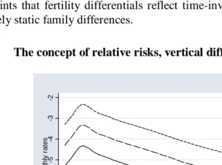
the fertility rates r1(t) to the time dimension of t for a group of women having another child, the dashed line describes r2(t) for another group, and the dotted line describes

) (

3 t

r for a third group—all on the scale of logged monthly rates. The relationship between the three lines imposed by the “relative-risks” specification can thus be specified as:

2 3 1 2

1() log () log ()

logr t = r t +c = r t +c (4),

where

c

c

scale. Equation 4 is a special case of the expression in Equations 3 and 3a. The “relative-risks” specification implies that fertility rates are always higher for one group than for the other group at any given time. In other words, time dependence is uninformative and irrelevant in comparing fertility rates. This approach thus imposes the constraints that fertility differentials reflect time-invariant behavioral mechanisms and relatively static family differences.

Figure 1: The concept of relative risks, vertical differences

-2

-3

-4

-5

-6

-7

-8

-9

lo

gg

ed

m

o

nt

hl

y

r

a

te

s

0 12 24 36 48 60 72 84 96 108 120 time

Figure 1: The Concept of Relative Risks, Vertical Differences

Note: The vertical differences between the groups are 1 on the logged scale. Formally, this can be written as,

2 ) ( log 1 ) ( log ) (

Figure 2: The concept of pace, horizontal shifts

-2

-3

-4

-5

-6

-7

-8

-9

lo

gge

d m

ont

h

ly

r

a

te

s

0 12 24 36 48 60 72 84 96 108 120 time

Figure 2: The Concept of Pace, Horizontal Shifts

Note: The horizontal difference between groups is consistently 12 months. Formally, this can be written as

) 24 ( log ) 12 ( log ) (

logr₁t = r₂t− = r₃t− , where group 1 is indicated by the solid line on the left, group 2 by the dashed line in the middle, and group 3 by the dotted line on the right.

In this paper, I adopt an alternative approach that models the “pace” of fertility. Unlike the “relative-risks” approach, which only shifts a hazard curve vertically, the “pace” approach represents a different conceptualization of fertility differentials by sliding a hazard curve horizontally to the right or to the left (see Coale and McNeil 1972, for the classic predecessor in demography; and Wu 2003, for a concise illustration of the concept). Figure 2 illustrates the “pace” specification, and the corresponding relationships between the solid line, r₁'(t), dashed line, r₂'(t), and dotted line, )r3'(t , can be written as:

) ' ( ' log ) ' ( ' log ) ( '

logr₁ t = r₂ t+c₁ = r₃ t+c₂ (5).

crossing). Under this approach, fertility differentials reflect behavioral mechanisms and family processes that are time contingent. 3

Not only do these two approaches reflect distinct behavioral mechanisms and family processes, they also differ in their implications for population dynamics through completed cohort fertility. The “relative-risks” approach of Figure 1 implies that

unequal proportions of women represented by the three lines will eventually give birth

to another child, whereas the “pace” approach in Figure 2 implies that equal proportions of women will give birth to another child—with only the “equilibrium proportions” reached at different durations. This statement can be confirmed either intuitively by comparing the areas under the three lines in Figure 1 and Figure 2, or formally via Equation 6 using the estimated fertility rate,

r

(t

)

  

 ⋅ − −

=

_∫

0

) ( exp 1 )

Pr(birth r t dt (6).

The proportion of women ever having another birth, Pr(birth), at a given birth order comprises the familiar concept of parity progression ratio in demography, thereby directly translating into the completed cohort fertility, a key element of cohort size (Ryder 1986). Substantively, this means that a sheer change in “pace” will not affect the completed cohort fertility and there will be no change in the population size of a cohort. However, an increase in “relative-risks” will increase the completed cohort fertility, and in turn increase population size. The discussion in this section suggests that the results presented in this paper may potentially help us speculate on how changing prevalence of stepfamilies may affect the future size of the U.S. population under distinct fertility regimes as modeled respectively by these two different approaches.

3. Method

3.1 Data and variables

Data come from the June Supplement of the 1995 Current Population Survey (CPS), which consists of a large nationally representative sample of households residing in the continental United States. The June 1995 CPS collected retrospective event history data concerning the first four and the most recent births and the first three and the most recent marriages for women between ages 15 and 65. The quality of these data is generally high (Bumpass 1983; Wu, Martin, and Long 2003), though there are relatively high inconsistencies in event histories for order marriages and higher-order births. Women who have had more than two marriages and more than four births may have preferences for large family size or lack the intention or ability to maintain a marital relationship, a potential source of unobserved heterogeneity that can bias the results. Women with more than two marriages and more than four births are thus excluded from the analytic sample to avoid biases due to data quality and unobserved heterogeneity—which require additional statistical and behavioral assumptions. Furthermore, the CPS did not collect any information on cohabiting unions and the fertility history of male partners.

The dependent variable is specific fertility rate. The female parity-configuration definition of stepfamily (see section 2.3) requires two independent variables: the number of children a woman has had in her lifetime (i.e., lifetime birth order or lifetime parity), and the number of children a woman has had in her current marriage (i.e., marital birth order or marital parity). The parity-specific fertility rates at time t can be formally defined as:

∆ ≥ ∆ + < ≤ =

+ → ∆

) | Pr(

lim ) (

0

t T t T t t

r (7).

3.2 Childbearing patterns: smoothed nonparametric fertility rates

The present analysis uses a nonparametric smoother of hazard rates developed by Wu (1989) to describe women’s childbearing patterns by both the number of children a woman has had in the current marriage and the number of children a woman has had in her lifetime. The reason I compare the childbearing patterns using fertility rates rather than the proportions of women having another child is that the time-dependent patterns of fertility rates preserve the richest amount of information, thereby allowing the analyst to infer the underlying behavioral mechanisms and family processes at work (Cox and Oakes 1984:16).

Wu’s (1989) method begins with a nonparametric hazard estimator, assuming a constant rate for t in the small interval, [tj−1,tj), based on the following joint likelihood function for events and censored cases (Cox and Oakes 1984):

j j j j j j j j j

j t t t

R C N C N t N t

r _ ≤ <

      + − ⋅ + ∆ − =

= log 1 , −1

) (

ˆ ) (

ˆ ρ , (8),

and j j j j j j j j j j

censor t t t

R C N C N t C t

r ≤ <

        + − ⋅ + ∆ − =

= log 1 , −1

) (

ˆ ) (

ˆ λ , (8a),

where Nj, Cj, Rj denote, respectively, the number of individuals who experience the

event, who are censored, and who are at risk of an event in the interval [tj−1,tj). This nonparametric estimator is a more general form of the standard life-table estimator in demography in that the life-table estimator is an approximation to this estimator (Equations 8 and 8a) via a Taylor series.

changing second derivative) or a changing variability of ρˆ with t. To increase j reliability, each interval of [tj−1,tj) contains at least ten events (Nj≥10). For tj

running through the entire marriage durations and birth intervals where we have data while requiring each tj containing ten or more events, this method demands a tremendous amount of data. This potential limitation is largely remedied by the large sample size of CPS, a major advantage over other data sets with marital and fertility history data. This method imposes substantially weaker statistical and behavioral assumptions, compared to alternative modeling approaches, though it should be considered as an exploratory rather than a confirmatory analysis. Thus, not only are the analyst’s theoretical preconceptions less likely to interfere with the results, the results obtained by this method will also be more resistant to biases caused by violated statistical assumptions.

4. Results

4.1 Descriptive statistics: parity definition of stepfamily status

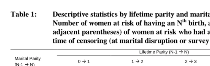
Table 1 presents basic descriptive statistics of the analytic sample and illustrates how combinations of marital parity and lifetime parity define stepfamily status. The first pair of columns in the first row indicates that 27,672 women were at risk of having a first lifetime child in their current marriage. Such births were, by the parity-configuration definition of stepfamily status in this paper, born to women in intact families because no children were born before their current marriage, whereby their lifetime parity equals their marital parity ( l m

P

Table 1: Descriptive statistics by lifetime parity and marital parity:

Number of women at risk of having an Nth birth, and percentage (in

adjacent parentheses) of women at risk who had an Nth birth by the

time of censoring (at marital disruption or survey interview)

Lifetime Parity (N-1 N) Marital Parity

(N-1 N) 0 1 1 2 2 3 3 4

0 1 27,672 (77%) 4,377 (56%) 2,665 (31%) 1,209 (23%)

1 2 21,005 (75%) 2,423 (44%) 804 (36%)

2 3 15,669 (46%) 1,066 (36%)

3 4 7,305 (42%)

Source: June Supplement, U.S. Current Population Survey, 1995 Note: Intact families (i.e., if marital parity = lifetime parity) are in bold face.

Descriptive statistics for stepfamilies are off diagonal. The second column of the first row indicates that there were 4,377 women at risk of having a second birth in their lifetime, but this child would be the first one in their current marriage. Note that the lifetime parity of these women is greater than their marital parity (Pl >Pm) and thus they were in a stepfamily when giving the birth. Similarly, the next column in the first row shows that, of the 2,655 women who had two children before their current marriage and were at risk of having their third lifetime birth and their first marital birth, 31% of them had done so.

The rest of the Results section presents the main substantive findings of this paper. Figures 3 through 11 present the results of comparing childbearing behaviors between intact families and stepfamilies at different marital and lifetime parities, as described in Table 1. The first three figures (Fig. 3-5) compare fertility rates among lifetime parities, holding marital parity constant. The next three figures (Fig. 6-8) compare fertility rates among marital parities, holding lifetime parity constant. The last three figures (Fig. 9-11) demonstrate the results using the “pace” approach.

4.2 Social norms of childbearing

lines in Figure 4 and Figure 5 represent fertility rates along the duration since last birth, for second marital births and third marital births, with all solid lines indicating intact families and dashed/dotted lines indicating stepfamilies. These lines follow the same unimodal shape, except that they peak later (at about one-and-a-half years for births in stepfamilies and about three years for intact families at all parities) than fertility rates for first marital births.

Figure 3: First births in a marriage by lifetime parity

-2 -3 -4 -5 -6 -7 -8 -9 s m o o thed l o gged mo nthl y fer ti lit y r a tes

0 12 24 36 48 60 72 84 96 108 120

marital duration in month

1st lifetime birth (intact fam) 2nd lifetime birth (stepfamily) 3rd lifetime birth (stepfamily) 4th lifetime birth (stepfamily) Figure 3: First Births in a Marriage by Lifetime Parity

Figure 4: Second births in a marriage by lifetime parity

-2 -3 -4 -5 -6 -7 -8 -9 s m o o th ed l o gg ed m o n thl y f e rt il it y r a te s

0 12 24 36 48 60 72 84 96 108 120 birth interval in month

2nd lifetime birth (intact fam) 3rd lifetime birth (stepfamily) 4th lifetime birth (stepfamily)

Figure 5: Third births in a marriage by lifetime parity

-2

-3

-4

-5

-6

-7

-8

-9

s

m

oot

hed l

ogg

ed

m

o

nt

hl

y

f

e

rt

ilit

y

r

a

te

s

0 12 24 36 48 60 72 84 96 108 120

birth interval in month

3rd lifetime birth (intact fam) 4th lifetime birth (stepfamily) Figure 5: Third Births in a Marriage by Lifetime Parity

The similarity in the qualitative shape of time dependence in fertility rates suggests that there may exist social norms for the timing of childbearing that are similar in both intact families and stepfamilies. Women tend to conceive a child as soon as they enter a marriage, as shown in the rates of first marital births peaking around one year of marriage duration in Figure 3. This result also shows how marriage is behaviorally “endogenous” to childbearing in that, first, the modal timing for a conception is close to the wedding (i.e., a honeymoon effect) and, second, the nonzero fertility rates within nine months of marriage are consistent with legitimizing intents of these women (i.e., shotgun marriages). Figures 4 and 5 are consistent with social norms for child spacing, with the ideal interval of having an additional child at three years for women in intact families and one-and-a half for women in stepfamilies—sooner than women in intact families.

Note also that the solid lines are always above the dashed/dotted lines in Figures 3 through 5. This indicates that the fertility rates for women in intact families are higher than the fertility rates for women in stepfamilies at any given marital parity. This is not a surprising finding, considering that at the same marital parity women in intact families are, by the definition of stepfamily (_Pl _>Pm

proportion of women stop childbearing once they have two children. The results also show no difference between intact families and stepfamilies in the fertility level gradients, implying that the empirical regularities depend primarily on a woman’s lifetime parity, not on her marital parity or stepfamily status.

4.3 Lifetime parity as fertility determinant and the “institutionalization hypothesis”

Figure 6: Second lifetime births by marital parity -2 -3 -4 -5 -6 -7 -8 -9 s m o o thed lo g g e d monthl y fe rt ili ty r a tes

0 12 24 36 48 60 72 84 96 108 120 marital duration or birth interval in month

2nd marital birth (intact fam) 1st marital birth (stepfamily) Figure 6: Second Lifetime Births by Marital Parity

Figure 7: Third lifetime births by marital parity

-2 -3 -4 -5 -6 -7 -8 -9 s m oothed lo g g e d mo n thl y fer ti lit y r a tes

0 12 24 36 48 60 72 84 96 108 120 marital duration or birth interval in month

3rd marital birth (intact fam) 1st marital birth (stepfamily) 2nd marital birth (stepfamily)

Figure 8: Fourth lifetime births by marital parity

-2

-3

-4

-5

-6

-7

-8

-9

s

m

o

o

th

e

d

l

o

g

g

ed m

ont

hl

y

f

e

rt

il

it

y

r

a

te

s

0 12 24 36 48 60 72 84 96 108 120 marital duration or birth interval in month

4th marital birth (intact fam) 1st marital birth (stepfamily) 2nd marital birth (stepfamily) 3rd marital birth (stepfamily) Figure 8: Fourth Lifetime Births by Marital Parity

4.4 The “pace” of fertility and the “institutionalization hypothesis”

Figure 9: Shift first marital birth by 36 months, second lifetime births by marital parity

-2 -3 -4 -5 -6 -7 -8 -9 s m o o the d lo gg ed m o n thl y f e rt il it y r a te s

0 12 24 36 48 60 72 84 96 108 120 marital duration or birth interval in month

2nd marital birth (intact fam) 1st marital birth (stepfamily) shifted 1st marital birth by 36 months

Second Lifetime Births by Marital Parity

Figure 9: Shift 1st Marital Birth by 36 Months

Figure 10: Shift first marital birth by 36 months, third lifetime births

by marital parity

-2 -3 -4 -5 -6 -7 -8 -9 s m ooth e d l o g ged m o nthl y f e rt il ity r a tes

0 12 24 36 48 60 72 84 96 108 120 marital duration or birth interval in month

3rd marital birth (intact fam) 1st marital birth (stepfamily) 2nd marital birth (stepfamily) shifted 1st marital birth by 36 months

Third Lifetime Births by Marital Parity

Figure 11: Shift first marital birth by 36 months, fourth lifetime births by marital parity

-2

-3

-4

-5

-6

-7

-8

-9

s

m

o

o

th

e

d

lo

gg

ed

m

o

nt

hl

y

f

e

rt

ili

ty

r

a

te

s

0 12 24 36 48 60 72 84 96 108 120 marital duration or birth interval in month

4th marital birth (intact fam) 1st marital birth (stepfamily) 2nd marital birth (stepfamily) 3rd marital birth (stepfamily) shifted 1st marital birth by 36 months

Fourth Lifetime Births by Marital Parity

Figure 11: Shift 1st Marital Birth by 36 Months

The identical right-tails of the fertility lines in Figures 9 through 11 suggest that the first marital births in stepfamilies have the same level and timing of fertility as the second and higher-order marital births in intact families or “institutionalized” stepfamilies at longer durations. This also provides complementary evidence that stepfamily’s adjustment towards an institutionalized union is a continuous process since its formation (as couples gradually have a first marital child as indicated by the right-tails), rather than a discrete process that begins only after the first marital child is born.

4.5 Implications for completed cohort fertility

completed cohort fertility due to the diminishing pattern at the early stage of fertility schedules for their first marital births.4 The fertility penalty for stepfamily women is different from the fertility penalty of marital disruption because not all divorced women remarry, but it specifically addresses the question whether increasing prevalence of stepfamily will increase the population size through increasing completed fertility. It is also important to qualify these results that the fertility penalty occurs only when women in stepfamilies have their first marital births. While not all stepfamilies survive long enough to become institutionalized, it is difficult to discern whether this implies unobserved heterogeneity among stepfamilies or an “incomplete institutionalization” effect. However, for stepfamilies that survive and move on to have their second and higher-order births in the marriage, the finding that levels and timings of fertility are identical in intact families and stepfamilies corroborates the institutionalization hypothesis.

4.6 Speculations on the constant thirty-six month “pace” difference

The pace differences between the first marital births in stepfamilies and all other births amount to a constant of thirty-six months. This finding presents an intriguing empirical regularity, for which this section offers two preliminary speculations of what it reveals. From the child’s perspective, the finding implies that when a stepchild (entering a new marriage with her/his mother) has a younger (half-) sibling, s/he will be thirty-six months older than if s/he were in an intact family. From the mother’s perspective, the thirty-six month difference reflects a “catch-up” effect. As illustrated in Figure 12, a woman’s normal life course of having another child in an intact family (top panel) is interrupted by separation, divorce, and remarriage when she takes a non-traditional trajectory for having a child in a stepfamily (bottom panel). She may be motivated to compensate for her lost reproductive time in the process of marital disruption and reconstitution by having a child at a faster pace when she enters a stepfamily. This motivation to “catch up” also appears in an earlier finding that the normative child spacing is about half the time in stepfamilies (one-and-a-half years) than it is in intact families (three years).

Figure 12: Decomposition of marital disruption and reconstitution in women’s life course of childbearing (top panel: uninterrupted childbearing for women in intact families; bottom panel: interrupted childbearing for women in stepfamilies)

5. Discussion

Nonparametric fertility rates in both intact families and stepfamilies appear to be highly regular. These regularities may imply normative beliefs regarding childbearing. Peaks of fertility rates for first marital births at around one year since the commencement of the marriage imply that women marry to have a child (i.e., marriage is “endogenous” to childbearing). The similar unimodal shape of fertility rates in all births reflects an ideal interval for child spacing. These empirical regularities are foundations for modeling fertility rates using any parametric or semi-parametric models on which future research may potentially build. The patterns also set the foundation for answering the main research question posed in this paper: How do childbearing behaviors compare between women in stepfamilies and in intact-families?

Results reported in this study suggest that, starting from the later stage in the process of having a first marital birth and continuing to second and higher-order marital births, the level and timing of fertility are identical in intact families and stepfamilies at any given lifetime parity. This finding supports the “institutionalization hypothesis” in childbearing behaviors, as the recent literature on stepfamily processes have documented in other behavioral domains (see Section 2.2 and Coleman et al. 2000). The empirical regularities in fertility rates highlight the importance of birth order in

Lifetime Parity N

Separation Divorce

Lifetime Parity N+1

Lifetime Parity N+1 Remarriage

fertility analysis, while suggesting lifetime parity, instead of marital parity or stepfamily status, is the primary determinant of fertility for American women.

The only differences found in the childbearing behaviors between intact families and stepfamilies are the “fertility penalty” at an earlier stage of stepfamily and the thirty-six month difference in the pace of fertility, both of which are unique to first marital births in stepfamilies. This “fertility penalty” finding complements the existing literature that shows remarried women have a lower completed fertility than the continuously married women (see the review in Section 2.1). Such results suggest that this differential may be either due to lowered fertility or indirectly due to higher marital instability, though only when a first marital birth occurs in the early stage of a stepfamily. This finding contradicts another sensible speculation that women bearing a first marital child in a stepfamily may have a higher completed fertility than the continuously married (through, e.g., conferring the subjective value of the couple’s commitment to the marriage), thereby a society may end up with a larger cohort size if the prevalence of stepfamilies increases at the population level.

The constant thirty-six month “pace” difference in fertility at all lifetime parities is a unique discovery using the “pace” modeling approach. We might make sense of this finding from the child’s perspective that the average age of obtaining a younger sibling is three years older for a stepchild than for a child in an intact family, and from the mother’s perspective that the lost reproductive time for a woman experiencing a marital disruption and reconstitution is approximately three years. Both speculations corroborate empirical facts reported in the literature. Bumpass (1984b) and Bumpass and Rindfuss (1979) estimated that, consistent with the child’s perspective, the median duration between parental separation and mother’s remarriage is about four years. Hetherington and Kelly (2002) reported that, consistent with the mother’s perspective, the respondents in their Virginia sample experienced roughly two years of psychological distress and economic difficulty after marital disruption before they were ready again to engage in an intimate relationship or to consider a new marriage. Nevertheless, these interpretations are oversimplified, and readers will note, from Figure 12, that the thirty-six month difference is indeed the convolution of waiting times in the additional transitions in the bottom panel, which requires estimates of all these transition rates and is thereby worthy of further investigation.

estimates of fertility rates not only avoid misspecification biases in the parametric models but also look into temporal patterns of childbearing behaviors as the family evolves. These results reveal empirical regularities that are informative of behavioral mechanisms and family processes, few of which can be readily derived from existing theories of stepfamilies or fertility alone.

The focus in this paper on the time dependence of fertility rates also provides an alternative analytic approach based on the “pace” of fertility to the conventional approach, which tends to use one coefficient to summarize the fertility differential. The “pace” approach, combined with the nonparametric procedure used in this paper, may have a greater potential for revealing complex motivational and behavioral mechanisms, despite the substantial appeal of a simple answer to whether an average woman in a stepfamily bears more children than her counterpart in an intact family. Relying on the strength of the “pace” approach, results reported in this paper unravel both the complexity and the regularity of childbearing behaviors at various stages (as indicated by the combinations of women’s parities) of intact families and stepfamilies.

Nonetheless, the conventional approach allows the analyst to control for confounding factors and thus has the power to formally adjudicate causal hypotheses, whereas the alternative approach is restricted to descriptive and exploratory purposes. Interpretation of the results also demands caution so as to distinguish between “unobserved heterogeneity” and “state dependence” (Heckman 1991; Vaupel and Yashin 1985). For example, the fertility penalty for first marital births in stepfamily may reflect either selective attrition of unstable marriages or difference in fertility behaviors. The empirical results reported in this paper do not allow us to determine which hypothesis carries more weight.

resolve the issue of how not to double count stepchildren—namely, once in the stepfamily formed by their biological father and again in the stepfamily formed by their biological mother—if the substantive interest is, as this paper purports to represent, the linking of family change to fertility and, ultimately, to population dynamics. Finally, the analysis conducted here does not distinguish among stepchildren born to a previously disrupted marriage and stepchildren born out of wedlock. Indeed, some of the out-of-wedlock births may be born to the same parents who later marry and continue to have more children. Hence, they are considered as stepchildren in this analysis, but not as stepchildren in the common sense. Those women who have had out-of-wedlock births may be different in their beliefs regarding marriage and family life, and their childbearing behaviors may not follow the same institutionalization process, though such limitations may be addressed in future investigations.

6. Acknowledgements

References

Bernstein, A. C. 1989. Yours, Mine, and Ours: How Families Change When Remarried

Parents Have a Child Together. New York: Macmillan.

Bogenschneider, K. 1997. “Parental Involvement in Adolescent Schooling: A Proximal Process with Transcontextual Validity.” Journal of Marriage and the Family 59: 718-33.

Booth, A. and J. N. Edwards. 1992. “Starting Over: Why Remarriages Are More Unstable.” Journal of Family Issues 13:179-94.

Buber, I. and A. Prskawetz. 2000. “Fertility in Second Unions in Austria: Findings from the Austrian FFS.” Demographic Research 3(2).

Bumpass, L. L. 1983. “The Comparability of Fertility and Marital Histories cross Fertility Surveys and Current Population Surveys.” CDE Working Paper 83-9. University of Wisconsin-Madison, WI.

———. 1984a. “Some Characteristics of Children's Second Families.” American

Journal of Sociology 90:608-23.

———. 1984b. “Children and Marital Disruption: A Replication and Update.”

Demography 21:71-82.

———. 1990. “What's Happening to the Family? Interactions between Demographic and Institutional Change.” Demography 27:483-98.

Bumpass, L. L., R. K. Raley, and J. A. Sweet. 1995. “The Changing Character of Stepfamilies: Implications of Cohabitation and Nonmarital Childbearing.”

Demography 32:425-36.

Bumpass, L. L. and R. Rindfuss. 1979. “Children's Experience of Divorce.” American

Journal of Sociology 85:49-65.

Casper, L. M. and S. M. Bianchi. 2002. Continuity and Change in the American

Family. Thousand Oaks, CA: Sage Publications.

Castro Martin, T. and L. L. Bumpass. 1989. “Recent Trends in Marital Disruption.”

Demography 26:37-51.

Chen, K. H., S. M. Wishik, and S. Scrimshaw. 1974. “Effects of Unstable Sexual Unions on Fertility in Guayaquil, Ecuador.” Social Biology 21:353-59.

Cherlin, A. J. 1978. “Remarriage as an Incomplete Institution.” American Journal of

Clarke, S., I. Diamond, K. Spicer, and R. Chappell. 1993. “The Relationship between Marital Breakdown and Childbearing in England and Wales.” Studies on

Medical and Population Subjects 55:123-36.

Coale, A. and D. R. McNeil. 1972. “The Distribution by Age of the Frequency of First Marriage in a Female Cohort.” Journal of the American Statistical Association 67:743-49.

Cohen, S. B. and J. A. Sweet. 1974. “The Impact of Marital Disruption and Remarriage on Fertility.” Journal of Marriage and the Family 36:87-96.

Coleman, M., L. Ganong, and M. Fine. 2000. “Reinvestigating Remarriage: Another Decade of Progress.” Journal of Marriage and the Family 62:1288-307.

Cox, D. R. and D. Oakes. 1984. Analysis of Survival Data. London: Chapman and Hall.

Downing, D. C. and D. Yaukey. 1979. “The Effects of Marital Dissolution and Re-Marriage on Fertility in Urban Latin America.” Population Studies 33:537-47.

Ebanks, G. E., P. M. George, and C. E. Nobbe. 1974. “Fertility and Number of Partnerships in Barbados.” Population Studies 28:449-61.

Friedman, J. H. 1984. “A Variable Span Smoother.” Technical Report No. 5. Department of Statistics, Stanford University, Stanford, CA.

Furstenberg, F. F. Jr. and G. B. Spanier. 1984. Recycling the Family: Remarriage After

Divorce. Newbury Park, CA: Sage.

Griffith, J. D., H. P. Koo, and C. M. Suchindran. 1985. “Childbearing and Family in Remarriages.” Demography 22:73-88.

Henz, U. 2002. “Childbirth in East and West German Stepfamilies: Estimated Probabilities from Hazard Rate Models.” Demographic Research 7(6).

Heckman, J. J. 1991. “Identifying the Hand Of The Past: Distinguishing State Dependence from Heterogeneity.” American Economic Review 81:75-79.

Hetherington, E. M. and J. Kelly. 2002. For Better or For Worse: Divorce

Reconsidered. New York: W. W. Norton.

Lauriat, P. 1969. “The Effect of Marital Dissolution on Fertility.” Journal of Marriage

and the Family 31:484-93.

Lillard, L. A. and L. J. Waite. 1993. “A Joint Model of Marital Childbearing and Marital Disruption.” Demography 30:653-81.

Loomis, L. S. and N. S. Landale. 1994. “Nonmarital Cohabitation and Childbearing among Black and White American Women.” Journal of Marriage and the

Family 56:949-62.

MacDonald, W. L. and A. DeMaris. 1995. “Remarriage, Stepchildren, and Marital Conflict: Challenges to the Incomplete Institutionalization Hypothesis.” Journal

of Marriage and the Family 57:387-98.

McCarthy, J. 1978. “A Comparison of the Probability of the Dissolution of First and Second Marriages.” Demography 15:345-60.

O’Connor, T. G., E. M. Hetherington, and D. Reiss. 1998. “Family Systems and Adolescent Development: Shared and Nonshared Risk and Protective Factors in Nondivorced and Remarried Families.” Development and Psychopathology 10:353-75.

Papernow, P. L. 1984. “The Stepfamily Cycle: An Experiential Model of Stepfamily Development.” Family Relations 33:355-63.

———. 1993. Becoming a Stepfamily: Patterns of Development in Remarried Families. San Francisco, CA: Jossey-Bass.

Peek, C. W., N. J. Bell, T. Waldren, and G. T. Sorell. 1988. “Patterns of Functioning in Families of Remarried and First-Married Couples.” Journal of Marriage and the

Family 50:699-708.

Ryder, N. B. 1986. “Observations on the History of Cohort Fertility in the United States.” Population and Development Review 12:617-43.

———. 1997. “Reflections on Reproductive Institutions.” Population and Development

Review 23:639-45.

Stewart, S. D. 2002. “The Effect of Stepchildren on Childbearing Intentions and Births.” Demography 39:181-97.

Thomson, E. 1997. “Her, His and Their Children: Influences on Couple Childbearing Decisions.” NSFH Working Paper No. 76. University of Wisconsin, Madison, WI.

———. 2004. “Stepfamilies and Childbearing Desires in Europe.” Demographic

Thomson, E., J. M. Hoem, A. Vikat, I. Buber, A. F. Prskawetz, L. Toulemon, U. Henz, A. L. Godecker, and V. Kantorova. 2002. “Childbearing in Stepfamilies: Whose Parity Counts?” In Fertility and Partnership in Europe: Findings and Lessons

from Comparative Research, Volume II, edited by E. Klijzing and M. Corijn.

New York: United Nations.

Thomson, E. and J.-C. A. Li. 2002. “Her, His and Their Children: Childbearing Intentions and Births in Stepfamilies.” NSFH Working Paper No. 89. University of Wisconsin-Madison.

Thornton, A.1978. “Marital Dissolution, Remarriage, and Childbearing.” Demography 15:361-80.

Toulemon, L. 1997. “The Fertility of Step-Families: The Impact of Childbearing before the Current Union.” Paper presented at the annual meetings of the Population Association of America, Washington, DC.

Vaupel, J. W. and A. I. Yashin. 1985. “Heterogeneity’s Ruses: Some Surprising Effects of Selection on Population Dynamics.” American Statistician 39: 176-85.

Vemer, E., M. Coleman, L. H. Ganong, and H. Cooper. 1989. “Marital Satisfaction in Remarriage: A Meta-Analysis.” Journal of Marriage and the Family 51:713-25.

Vikat, A., E. Thomson, and J. M. Hoem. 1999. “Stepfamily Fertility in Contemporary Sweden: The Impact of Childbearing before the Current Union.” Population

Studies 53:211-25.

Vikat, A., E. Thomson, and A. Prskawetz. 2004. “Childbearing Responsibility and Stepfamily Fertility in Finland and Austria.” European Journal of Population 20:1-21.

Vuchinich, S., E. M. Hetherington, R. Vuchinich, and G. G. Clingempeel. 1991. “Parent-Child Interaction and Gender Differences in Early Adolescents’ Adaptation to Stepfamilies.” Developmental Psychology 27:618-26.

Vuchinich, S., R. Vuchinich, and B. Wood. 1993. “The Interparental Relationship and Family Problem-Solving With Preadolescent Males.” Child Development 64:1389-400.

Waldren, T., N. Bell, C. Peek, and G. Sorell. 1990. “Cohesion and Adaptability in Post-Divorce Remarried and First-Married Families: Relationships With Family Stress and Coping Styles.” Journal of Divorce and Remarriage 14:13-28.

Wineberg, H. 1990. “Childbearing after Remarriage.” Journal of Marriage and the

Family 52:31-38.

———. 1992. “Childbearing and Dissolution of the Second Marriage.” Journal of

Marriage and the Family 54(4):879-87.

Wu, L. L. 1989. “Issues in Smoothing Empirical Hazard Rates.” Sociological

Methodology 19:127-59.

———. 2003. “Event History Models for Life Course Analysis.” Pp. 477-502 in

Handbook of the Life Course., edited by Jeylan T. Mortimer and Michael J.

Shanahan. New York: Kluwer Academic.

Wu, L. L. and J.-C. A. Li. 2005. “Historical Roots of Family Diversity: Marital and Childbearing Trajectories of U.S. Women.” Pp. 110-49 in On the Frontier of

Adulthood: Theory, Research and Public Policy., edited by. R. A. Settersten, R.

G. Rumbaut, and F. F. Furstenberg. Chicago, IL: University of Chicago Press.