Volume 9 - Article 10 | Pages 223–262

in the population sciences published by the Max Planck Institute for Demographic Research Konrad-Zuse Str. 1, D-18057 Rostock · GERMANY www.demographic-research.org

DEMOGRAPHIC RESEARCH

VOLUME 9, ARTICLE 10, PAGES 223-262

PUBLISHED 13 NOVEMBER 2003

www.demographic-research.org/Volumes/Vol9/10/

DOI: 10.4054/DemRes.2003.9.10

Research Article

Elaboration of the Coale-McNeil

Nuptiality Model as the Generalized

Log Gamma Distribution:

A New Identity and Empirical

Enhancements

Ryuichi Kaneko

1 Introduction 224 2 Coale-McNeil Model and the Generalized Log

Gamma Distribution

225

2.1 Coale-McNeil Model 225

2.2 Coale-McNeil Model as The Generalized Log Gamma Distribution

228

3 The GLG Model as an Analytic Tool for First Marriage

231 3.1 Development of Country Specific Standard

Schedules

231 3.2 Estimation of Covariate Effects on First Marriage

Timing with/without Competing Risk Framework

236

4 Empirical Enhancement 239

4.1 Empirical Adjustment of the GLG Model 239

4.2 Method of Parameter Estimation 244

4.3 Censoring Effects on Parameter Estimation 245

5 Application of the Adjusted GLG Model 246

5.1 Estimation and Projection of First Marriage 246

5.2 Application for Fertility Projection 250

6 Summary and Conclusion 255

7 Acknowledgements 256

Notes 257

References 259

Research Article

Elaboration of the Coale-McNeil Nuptiality Model

as the Generalized Log Gamma Distribution:

A New Identity and Empirical Enhancements

Ryuichi Kaneko 1

Abstract

The Coale-McNeil nuptiality model is a particular case of the generalized log gamma distribution model. In this paper, we demonstrate that recognition of this connection allows an expansion of the possible applications of the Coale-McNeil model. As examples, we propose a procedure to develop country specific standard schedules, and illustrate the utility in regression analysis (directly and via the competing risk framework). In addition, we employ this identification to enhance the ability of the models with empirical adjustment to trace the trajectory of the lifetime schedule for cohorts which have not completed the process. We illustrate an application to Japanese female cohorts. We also propose an application to fertility projection by modeling the fertility schedule by birth order.

1

1. Introduction

The Coale-McNeil (CM) nuptiality model is a mathematical expression of regularity in age patterns of first marriage. It is a standard demographic tool for the estimation and projection of age schedules of first marriage and birth by birth order. However, it is not generally recognized by researchers that the CM model without a prevalence parameter is precisely the log version of the generalized gamma distribution with limited parameter space (Kaneko 1991a). Clear recognition of this connection is useful because it enables the utilization of the rich body of knowledge about the statistical properties of the generalized gamma distribution when pursuing demographic applications. Conversely, some of the analysis of the structure of the CM model (such as the interpretation of the convolution structure) can be applied to understanding the generalized log gamma distribution. The first purpose of this article is to demonstrate some of the demographic applications that benefit from this new description of the CM framework. We present algorithms for formalized development of country-specific standard schedules. In addition, we provide an analysis of the effects of covariates on marriage timing, both with and without application of the competing risk framework for different types of marriages.

2. Coale-McNeil Model and the Generalized Log Gamma

Distribution

2.1 Coale-McNeil Model

Following the finding by Coale (1971) that age specific rates of first marriages for female cohorts from different countries showed virtually identical patterns if location, scale, and eventual proportion of ever marrying are adjusted, Coale and McNeil derived a statistical distribution that described observed distributions of age at first marriage (Coale and McNeil 1972). The closed form description of the probability density function (PDF) for this distribution is:

(

)

{

(

)

}

( )

exp

exp

(

)

g x

β

α

x

µ

β

x

µ

α β

é

ù

=

_ë

−

−

−

−

−

_û

Γ

(1)

where

Γ

denotes the gamma function ( 1

0

( )

x

∞

t

x− −

e dt

t

Γ

=

_ò

),

α >

( 0)

,

β >

( 0)

, and

(

)

µ

−∞ < < ∞

µ

are three parameters (Coale and McNeil 1972). For practical application, they provided a standard marriage schedule model from a location-scale family of this distribution by fixing the shape according to the experiences of Swedish female cohorts. The following is an adjusted version of the standard model with mean zero, and variance unity by Rodriguez and Trussell (1980), obtained by setting

1.145,

1.896

α

=

β

=

, and

µ = −

0.805

in equation (1):

(

)

{

(

)

}

( ) 1.2813exp

=

é

_ë

−

1.145

+

.805

−

exp

−

1.896

+

.805

ù

_û

s

g z

z

z

. (2)

Let

g x

( )

denote a distribution of age at first marriage of any female cohort with its observed mean,

u

, standard deviation, b. Using the standard model above, it is given by:

1

( ; , )

≅

_s

(

x u

−

)

g x u b

g

b

b

(3)

( )

=

( )

f x

C g x

(4)

where C denotes proportion eventually marrying in the cohort. Thus, the age distribution underlies the age schedule (the age specific rate) with parameter of prevalence measure, C.

Clear definition of terms is essential. In this paper, the probability density

f x

( )

given by (4) is called first marriage schedule, the underlying distribution

g x

( )

in the same equation is called distribution of age at first marriage, and the normalized distribution with fixed shape

g x

_s

( )

given by (2) is the (global) standard distribution of age at first marriage. Thus,

C g x

_s

( )

is the (global) standard schedule.

An interesting feature of the CM distribution is that it is a limiting probability distribution of convolution of infinite set of mean-related exponential distributions. Thus, it is regarded as a convolution of distribution of its own form and some numbers of related exponential distributions as well. This structure provides a mathematical model for the multistage process, by which we mean a process that consists of multiple processes required for the target event to happen. In fact, Coale and McNeil (1972), inspired by Feeney (1972), viewed first marriage as a multistage process in which entry into marriageable state, meeting of the eventual spouse, and engagement are required to take place prior to the marriage.

Suppose we form the convolution of the m exponential distribution with parameter

α

,

α β

+

,

α

+

2

β

, …,

α

+

m

β

, where

α

and

β

are two parameters with positive real values, and let

h t m

_T

( ; )

denote PDF of the resulting distribution, then the CM distribution given in equation (1) is the convolution of two distributions whose PDFs are:

{

}

( ; )

exp

(

)(

) exp

(

)

(

)

=

é

_ë

− +

−

−

−

−

ù

_û

Γ

+

X

g

x m

m

x

x

m

β

_α

_β

_µ

_β

_µ

α β

(5)

(

)

{

}

1

( )

(

)

( ; )

1 exp

exp

(

)(

1)!

−

Γ

+

=

−

−

−

Γ

−

m

T

m

h t m

t

t

m

β α β

_β

_α

α β

(6)

stage from when the process starts, and

h t m

_T

( ; )

is the distribution of the waiting time that is composed of m exponentially distributed waiting times. The mean and variance

of distribution

g

_X

( ; )

x m

are respectively

−

1

æ

_ç

+

ö

_÷

è

m

ø

α

µ

ψ

β

β

, and

2

1

_′

æ

ö

+

ç

÷

è

m

ø

α

ψ

β

β

, where

ψ

and

ψ

′

are the digamma and trigamma functions. Those

of distribution

h x m

_T

( ; )

are respectively

{

}

1

1

(

1)

−

=

+

−

å

m

j

m

α

β

, and

{

}

2

1

(

1)

−

=

+

−

å

_jm

α

m

β

.

The exponential distribution with the three largest means convoluted in distribution

h t m

_T

( ; )

have the parameters

α

,

α β

+

, and

α

+

2

β

. For the first marriage process, Coale and McNeil supposed that these are distributions of duration from entry into the marriage market to the meeting of future husband, dating duration, and engagement duration. According to parameter values of the CM standard age distribution (2), which are derived from the experiences of Swedish female cohorts, the mean duration from entry into the marriage market to the meeting of future husband is estimated as (

1 0.174

) or 5.75 years. Similarly, means of the second and third waiting durations are 2.16 years (

1 (0.174 0.2881)

+

) and 1.33 years

(

1 (0.174 2 0.2881)

+ ×

) respectively (Coale and McNeil, 1972). However,

2.2 Coale-McNeil Model as The Generalized Log Gamma Distribution

Some authors have discussed relationships of the Coale-McNeil distribution to other well-known probability distributions. Coale and McNeil themselves pointed out that the CM distribution is the extreme value distribution (of type I, or equivalently the Gompertz distribution for non-negative random variables) when

α β

=

(Coale and McNeil, 1972). Rodriguez and Trussell discussed its relationships with the gamma distribution (Rodriguez and Trussell, 1980). Liang (2000) discussed its relationships to the extreme value, log-gamma, and the normal distribution based on discussion of the log-gamma distribution by Johnson et al. (1994). The conclusive observation on these relationships is that the CM distribution is precisely equivalent to the generalized log gamma (GLG) distribution with a somewhat different parameter space (Kaneko 1991a). This explains the relationships of the CM distribution to the extreme, the log gamma, and the normal distributions, since these arise as special cases of the generalized log gamma distribution.

The generalized gamma (GG) distribution was defined by Stacy (1962), introducing an additional parameter into the gamma distribution (Note 3). If a random variable follows the GG distribution, then the log-transform of the random variable follows the GLG distribution (some authors such as Johnson et al. 1994, call it the log generalized gamma distribution), which is a mirror image of the CM distribution reflected at the origin (

x

=

0

). Prentice (1974) proposed an alternative parameterization of the GLG distribution which extends the parameter space so as to express both mirror images of the distribution corresponding to random variable X and -X by one model. Hence, it includes the CM distribution as a constrained version with half of the extended parameter space. Here we refer to Prentice's extended version simply as the GLG distribution.

The PDF and the cumulative distribution function (CDF) of the GLG distribution are given by:

2

2 1 2

2

( )

(

)

exp

exp

(

)

−

− − −

−

é

æ

−

ö

ì

æ

−

ö

ü

ù

=

_ê

_ç

_÷

−

_í

_ç

_÷

_ý

_ú

Γ

_ë

_è

_ø

_î

_è

_ø

_þ

_û

x u

x u

g x

b

b

b

λ

λ

λ

λ

λ

λ

λ

(7)

2 2

( )

= −

1

æ

_ç

−

,

−

exp

æ

_ç

−

ö

_÷

ö

_÷

è

ø

è

ø

x u

G x

I

b

where

λ

(

−∞ < < ∞ ≠

λ

,

0),

u

(

−∞ < < ∞

u

),

b

( 0)

>

are three parameters, and

Γ

and

I

denote the gamma function and the incomplete gamma function respectively (Note 4). Parameter

λ

determines the shape of the distribution; if it is positive, the distribution is skewed to the left, and if it is negative, it is skewed to the right. The distribution is not defined for

λ

=

0

, but as

λ

→

0

, the distribution approaches the normal distribution.

u

is a location parameter which determines the location of the mode of the distribution.

b

is the scale parameter of the distribution.

The following alternative parameterization of the CM distribution allows representation of the full range of the parameter space as the GLG distribution:

(

)

_{

(

)

_}

( )

exp

exp

( )

é

ù

=

_ë

−

−

−

−

−

_û

Γ

g x

k

x

x

k

β

_β

_µ

_β

_µ

(9)

where

k

( 0)

>

is a new parameter, and

β

is now allowed to take a negative value (Note 5).

Since the original CM distribution corresponds to the GLG distribution with a negative value of

λ

, and we consider only situations in which

λ

takes on a negative value, we can regard the GLG distribution as equivalent to the CM distribution throughout the paper.

One of the advantages of the GLG formulation is that it has only one shape parameter, i.e.

λ

. Describing the shape of the distribution by a single value is quite useful in applications. Since it identifies a distribution once location and scale are controlled for, it can be regarded as an index of schedule shape specific to cohorts of a country or region, for instance. In fact, the essential nature of the CM global standard nuptiality schedule is constancy across population groups of the shape parameter at a value of

λ

–1.287. Substantial implication of the shape value is discussed later. In the next section, we describe a simple procedure to develop country specific standard schedules which takes advantage of the single shape parameter. The single shape parameter is quite effective in developing fertility schedules by birth order as well, since the shape value varies by birth order.

The mean and variance of the GLG distribution are respectively given as:

2 2

(

){ (

) ln

}

+

+

u

b

λ ψ λ

λ

(10)

2 2

The mode is simply u, with the maximum of PDF given by:

2 2

2

2

(

)

(

)

− − − − −

=

Γ

)

g

e

b

λ λ

λ

_λ

λ

.

As mentioned earlier, the GLG distribution includes many of the fundamental distributions as special cases. Specifically, it specializes to the extreme value distribution when

λ

=

1

, the (standard) log-gamma distributions when

,

2 ln

=

b u

= −

λ

λ

, and even the normal distribution as a limiting case when

0

→

λ

. These relations are a reflection of relationships between the GG distribution and the exponential, the Weibull, the gamma, and the log normal distributions, and it guarantees that the GLG distribution describes age distribution of first marriages better than those specialized distributions.

The correspondence between the parameters of the CM and GLG distributions can be expressed as:

1

= −

b

α

λ

,

= −

b

λ

β

,

µ

= −

u

b

ln

λ

2

λ

(12) or equivalently, 1 2 −

æ ö

= −

_{ç ÷}

è ø

α

λ

β

,

( )

1 2 −

=

b

αβ

,

= −

1

ln

æ ö

_{ç ÷}

è ø

u

µ

α

β

β

, (13)

where

α β

,

, and

µ

are parameters of the CM formulation in (1) (Kaneko 1991a). The revised version of the CM standard distribution of age at first marriage by Rodriguez and Trussell given by (2) is expressed by the GLG with parameters

1.287

= −

λ

,

u

= −

0.5390

,

b

=

0.6787

.

(

)

2

2 2 2

2

( ; ) ( ) exp exp

( ) − − + − − − é æ − ö ì æ − öüù = _ê + _{ç ÷}− _{í ç ÷ýú} Γ + _{ë è ø î è øþû} m X

x u x u

g x m m

b m b b

λ

λ

_λ

_λ

_λ

_λ

_λ

λ

(14) 1 2 2

(

)

( ; )

1 exp

exp

(

)(

1)!

− − −

Γ

+

ì

æ ö

ü

æ

ö

=

_í

−

_{ç ÷}

_ý

_ç

_÷

Γ

−

_î

_{è ø}

_þ

_è

_ø

m T

m

t

t

h t m

b

m

b

b

λ λ

λ

λ

λ

(15)

where the parameters are the same as given above and m is the number of the mean-related exponential distributions that compose the waiting time distribution

h x m

_T

( ; )

.

Theories, application frameworks, and computer software packages developed for either distribution can be applied to the other. This is particularly useful in view of the wide array of utilities for working with the GG and GLG distributions. In the following section, we first demonstrate the usefulness of the GLG formulation as an analytic tool for studying first marriage behavior, and then we conduct empirical enhancement of the applicability of the model to predict trajectories of marriage and fertility schedules.

3. The GLG Model as an Analytic Tool for First Marriage

3.1 Development of Country Specific Standard Schedules

The first demonstration of the usefulness of the new identification of the CM model exploits the feature that it has only one shape parameter (

λ

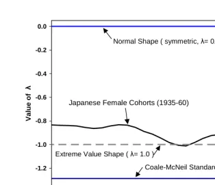
). This enables us to make country specific standard schedules through undemanding procedure. Country specific standards are sometimes required and often desirable, since the global standard schedule derived from Swedish experiences might be inappropriate for some populations. In addition, identifying the specific shape value to apply for a schedule is crucial for predicting the fertility by birth order, since the value for each order varies from that of the nuptiality standard. In the following, we illustrate the development of a country specific schedule using Japanese female cohorts.

Figure 1: Estimated Shape Parameter Values (λ) of The GLG Model For Japanese Female Cohorts born in 1935-60

Figure 1 shows the trend of parameter

λ

estimated for Japanese female cohorts born in 1935-1960 who have attained at least age 40 at the time of evaluation. The figure indicates deviations in the shape values of Japanese cohorts from the value of the CM standard schedule, which is derived from Swedish experiences. The shape values of Japanese cohorts fall in the range from –1.0 to –0.8, while it is at –1.287 for the CM standard. Other particular values correspond to well-known underlying distributions. The value zero corresponds to the normal distribution, and the value unity to the extreme value distribution. The shape values of Japanese cohorts are located in the middle of the CM standard and the normal distribution near the extreme value model, implying that the Japanese schedule is more symmetric than the CM standard. It seems a little more feasible to use the extreme value distribution to describe Japanese cohorts. We consider some of reasons for the symmetry seen in Japanese cohorts later. A mild decline in the shape value over cohorts is also identified in the figure.

-1.4 -1.2 -1.0 -0.8 -0.6 -0.4 -0.2 0.0

1935 1940 1945 1950 1955 1960

Year of Birth

V

a

lu

e

o

f

λ

Coale-McNeil Standard ( λ= -1.287 ) Normal Shape ( symmetric, λ= 0.0 )

Japanese Female Cohorts (1935-60)

Coale’s original finding about first marriage schedules is, in our translation, that the shape parameter of the age distribution is common over countries and periods (Coale 1971). It has been validated by the wide use of the shape-fixed CM standard schedule as a practical tool in various demographic applications. However, the stability of shape is, of course, an approximation. Our close examination indicates that it varies across countries (Japan is not the same as Sweden), and undergoes changes over time to some extent as well. Thus, a schedule with a shape value specific to Japanese women is expected to be more accurate. On the grounds that the shape characterizes the first marriage process of a nation, developing country specific standard schedule with an appropriate shape value is quite beneficial. Such a specific schedule offers more accuracy with the same general form. We now describe the procedure for producing a country specific shape-fixed standard schedule with mean zero and standard deviation of unity.

Let

λ

_s denote shape parameter of the GLG model which is specific to cohorts of a country. The following parameters are to be calculated for the new standard:

2

−

=

s s

k

λ

,

( )

'( ),

'( ),

'( )

=

=

=

s

s s s s s s

s

k

k

k

k

k

ψ

α

ψ

β

ψ

µ

ψ

, (16)

where

ψ

and

ψ

′

denote the digamma and trigamma function. Using these parameters, the underlying distribution of age at first marriage in the new standard schedule is given by:

(

)

{

(

)

}

( )

exp

exp

(

)

é

ù

=

_ë

−

−

−

−

−

_û

Γ

s

s s s s s

s s

g z

β

α

z

µ

β

z

µ

α β

(17)

The country specific shape value

λ

_s can be obtained by averaging values of

λ

of the GLG model fitted to source schedules. Then any first marriage or fertility distribution

( )

1

( )

=

_s

(

−

)

x x

x

x

g x

g

s

s

, (18)

( )

=

( )

f x

C g x

, (19)

where

x

and

s

_x are the mean and standard deviation of the distribution, and C is the proportion eventually marrying, of a target cohort.

For Japanese female cohorts born between 1935-60, the average of the estimated

λ

of the GLG model is -0.9123. With this value for

λ

_s, and following the formulas (16) and (17), our new Japanese female standard marriage schedule

g z

_j

( )

is given by:

(

)

{

(

)

}

( )

=

1.226 exp

_ë

é

−

1.351

+

0.2553

−

exp

−

1.125

+

0.2553

ù

_û

J

g

z

z

z

. (20)

Figure 2: Comparison of Japanese Standard Schedule with The Coale-McNeil Standard for First Marriage of Female Cohort

Searching for the determinants of the shape is essential for many applications of the model. As shown later, it is crucial to identify the shape in predicting the schedules of young cohorts that have yet to complete their process. As seen in Figure 1, the shape value changes over time. For example, if presence of arranged marriage makes the shape symmetric and proportion of arranged marriage decreases over time, the shape value is expected to approach that of the CM standard.

0.0 0.1 0.2 0.3 0.4 0.5 0.6

-3 -2 -1 0 1 2 3 4 5

Standardized Age

P

robabi

li

ty

D

e

nsi

ty

3.2 Estimation of Covariate Effects on First Marriage Timing with/without Competing Risk Framework

Though extensions to incorporate covariates into the CM model have been conducted by several authors (Trussell and Bloom 1983, Sørensen and Sørensen 1986, Liang, 2000), the GLG specification has some advantages for this purpose in both theoretical and practical developments since it is one of the standard parametric regression models in survival analysis (Lawless 1982, Johnson et al. 1994 1995, Klein and Moeschberger 1997). Here, we demonstrate the effectiveness of the model in analysis of covariate effects on age at first marriage, and the effect of heterogeneity on shape parameter value, which is significant in predicting the parameter required for nuptiality and fertility projection described later in this paper.

In the standard specification of the GLG regression model, a vector of covariates for individual i, Xi, are incorporated into the model in linear form with regression

parameters

θ

, so that the parameter u of equation (7) and (8) for individual i should be

=

X

t

θ

i i

u

where

X

t_i denotes the transpose of vector

X

_i. Since the parameter u determines the location of the schedules (the mode), the specification implies that individuals have underlying probabilities that differ in marriage or reproduction timing depending on their characteristics. This formulation is particularly useful for analysis of the current fertility decline to below replacement level in many countries, since the decline is firmly connected with delay in timing of marriage and childbearing.

We conduct the GLG regression for age at first marriage with some demographic and socio-economic characteristics using survey data for illustrative purposes (Note 6) (The source is the national representative sample in the Ninth National Fertility Survey conducted in 1987 in Japan). The results are presented in Table 1 in the far left two columns (“All Marriage”), where estimated parameter values and regression coefficients for two different model specifications (model 1 and 2) are shown.

Table 1: Effects of Covariates on Age at First Marriage of Japanese Women: The GLG Regression by Type of Marriage with Competing Risk Model

All Marriage

Covariates Model 1

(N=4682)

Model 2 (N=4682)

Non-Arranged (N=4682) (n=2878)

Arranged (N=4682) (n=1804)

Intercept 23.34 22.43 23.86 23.33

Cohort (Birth Year) **** ****

# 1938-39 0.00 0.00 0.00 0.00

1940-44 0.04 -0.05 -0.36 0.30

1945-49 0.17 -0.11 -0.72 *** 0.75 ***

1950-54 0.20 -0.18 -1.02 **** 1.29 ****

Educational Background **** **** ****

# Junior College 0.00 0.00 0.00

High School 0.87 **** 0.82 **** 0.89 ****

Junior College 1.49 **** 1.69 **** 1.00 ****

University 2.48 **** 2.61 **** 2.05 ****

Father's Occupation ** ** ***

# Agriculture 0.00 0.00 0.00

Self-employed 0.13 -0.10 0.50 **

White-colalr 0.17 -0.16 0.70 ****

Blue-collar -0.13 -0.49 ** 0.48 *

Not working/ temporary -0.44 * -0.69 ** 0.02

Area of Residence **** ****

# Rural 0.00 0.00 0.00

Urban 0.42 **** 0.13 0.98 ****

Co-residence with *** ****

# Living seperately 0.00 0.00 0.00

Living together 0.09

Heiress

# Not heiress 0.00 0.00 0.00

heiress -0.16 -0.06 -0.22

Number of Sibling -0.07 ** -0.12 0.04

Scale Parameter (b) 2.614 2.460 3.082 3.453

Shape Parameter (λ) -0.673 -0.761 -1.161 -1.054

N : Sample Size n : Number of Samples without Censor # : Reference Category * P<0.05 ** P<0.01 ***P<0.001 ****P<0.0001

While the effects of heterogeneity of individual characteristics in relation to first marriage timing are measured above, we next view the effects of heterogeneity of characteristics of marriage itself. There occur several different types of marriage such as non-arranged and arranged marriages, registered marriage and cohabitation, or inter-racial and intra-inter-racial marriages, and so forth. For instance, consider a situation in which the marriage processes of non-arranged and arranged marriages are to be compared. One plausible supposition here is that the same person goes through different processes simultaneously and ends up in either of these different types of marriage, whichever comes first. According to the survival analysis framework, this type of situation can be dealt with by the competing risk model, in which several different events have their own mutually independent probabilities of taking place at a given time.

We illustrate the use of the competing risk framework by applying it to analysis on determinants of first marriage timing in Japan taking into account the type of marriage, i.e. non-arranged and arranged marriage. The results are presented in the right two columns of Table 1. Here, some interesting tendencies hidden in the analysis of all over marriage appear. First, age at first marriage decreased by cohort for non-arranged marriages, while it increased for arranged marriages. These changes in opposite directions are both statistically significant and substantial in amount. On the other hand, as described before, the trend as a whole for all marriages indicates no significant change by cohort. The analysis by type of marriage here revealed active changes behind the seeming stability over the cohorts. Similar opposite effects by type of marriage are seen for some other covariates. Co-residence with parent(s) before marriage significantly affects marriage timing of each type in opposite directions (delay in the non-arranged, and accelerated in the arranged marriage) while that of over all marriage appears to be unaffected. Residence in urban areas delays only arranged marriage. Only non-arranged marriage is accelerated by the presence of siblings. The analysis illustrates that examination by type of marriage with the competing risk framework provides us with information about detailed features of the process which are otherwise not observable.

4. Empirical Enhancement

4.1 Empirical Adjustment of the GLG Model

No model fits actual data perfectly. Discrepancies consist of two types of errors; one is random error induced by exogenous factors such as measurement error, and the other is systematic error derived from simplification or insufficiency in model specification. The latter may be corrected by exploiting regularity in the pattern of error. Here we introduce empirical adjustments of the GLG model, seeking a better fit to actual experiences in first marriage of Japanese female cohorts.

The GLG model does not satisfactorily describe the first marriage experiences of Japanese female cohorts. This issue is partly discussed above, where the shape of the standard schedule is inappropriate and therefore is to be set to a specific value to create a country-specific schedule. But even allowing the shape parameter to take value specific to a target cohort, the model schedule deviates noticeably from the observed data. Figure 3 shows observed (dots) and modeled (broken line) first marriage rates for Japanese female cohorts born in 1950. Although the model is best-fitted by optimizing all parameter values including the shape value, the discrepancy is sizable. A similar error pattern is found for every cohort that completed the marriage process in our data set, and therefore the errors can be regarded as systematic. The discrepancy causes serious distortion in estimated parameter values especially when the model is applied to censored cohorts that have not completed their marriage processes. Therefore, seeking better fit for the model is critical in predicting eventual schedule of nuptiality and fertility for cohorts that have not completed the process.

To improve the predictive power of the model in this circumstance, we should capture regularity in the error pattern to be modeled. Difference in the cumulative first marriage rates by age between actual and fitted experiences for 16 cohorts (born in 1935 through 1950) that completed the marriage process are examined. We adjust the cumulative rate function instead of the first marriage rate function because the former is used in parameter estimation, as describe later.

Figure 4 shows the errors for the cohorts. In the figure, the horizontal coordinate is calibrated by standardized age z in terms of parameter u and b, i.e. with usual age x:

(

)

= −

(

, , ,

)

=

θ

C

λ

u b

are the cumulative function of the first marriage rate of observed and

model (the latter is alternatively represented by

F z

ˆ ( ; ),

θ θ

=

(

C

, , 0,1

λ

)

.)

As mentioned above, a highly systematic age pattern of error exists. It is reasonable to assume that there is a particular cause for the very persistent age pattern of discrepancy seen in Figure 4. However, here we just model the pattern empirically. We return to a discussion of underlying causes of the error pattern later.

The straightforward way to incorporate the error pattern into the model is to add an average error pattern to the model. The resulting model

F x

( ; ),

θ θ

=

(

C

, , ,

λ

u b

)

is expressed as:

ˆ

ˆ

( ; , , , )

=

( ; , , , )

+

æ

_ç

−

ö

_÷

è

ø

x u

F x C

u b

F x C

u b

b

λ

λ

ξ

, (21)

where

F x

ˆ ( ; )

θ

is the GLG model, and

ξ

ˆ z

( )

is the average error at standardized age z, called the adjustment function (Note 8). We call this model the empirically adjusted GLG model. Although incorporating empirical residual pattern into the mathematical model is not an elegant solution, the simple way out is of practical efficacy.

Figure 3: Observed Age Specific First Marriage Rates and Fitted GLG Model (with and without Adjustment): Japanese Female Cohort born in 1950

Figure 4: Errors of the GLG Model in Cumulative Fist Marriage Rate for Japanese

Female Cohort (1935-50) and Adjustment Function

-0.03 -0.02 -0.01 0.00 0.01 0.02 0.03 0.04 0.05

-4 -2 0 2 4 6 8 10

Standardized Age

Ra

te

Mark : errors Line : adjustment function

20 25 30 35 40 45 50

0.02 0.04 0.06 0.08 0.1 0.12 0.14

1950

Mark : observed

Solid Line : the GLG model (with adjustment) Broken Line : the GLG model (without adjustment)

F

ir

s

t M

a

rr

ia

g

e

R

a

te

In Figure 3, we see an improvement in the results produced by the adjusted model (solid line). The curve produced by the adjusted GLG model traces almost exactly the observed rates, while, as already mentioned, the GLG model without adjustment (broken line) does not (Note 9).

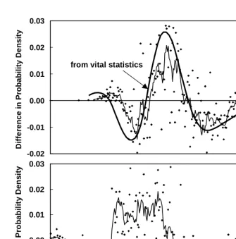
Now we briefly discuss the cause of the error pattern. The upper graph of Figure 5 shows the average error pattern in the first marriage rate of the Japanese female cohorts from vital statistics and from a national representative sample. Both patterns indicate that first marriages concentrate on the mode (age 23-24) more than is predicted by the GLG model. A similar error pattern is reported in attempts to fit the Coale-McNeil model to cohort experiences in other countries (for the U.S., Bloom and Bennett 1990, for Swedish male, Ewbank 1974). If the model should represent the “natural” course of first marriage schedule, people should exert a certain kind of regulation on age at marriage resulting in the error pattern. Since in the US, the actual rate exceeds the prediction of the model in the late teens, where the mode locates, Bloom and Bennett speculate that there is a threshold age of 18 before which marriage is hindered by laws or cultural norms. In our case in Japan, however, excess marriages concentrate on age 23-24. Inquiring as to the cause of this residual pattern, we might ask if age at marriage is regulated directly by couples or if the pattern is formed spontaneously in course of marriage process. We observe the error pattern of distribution of age at first encounter with eventual spouse through a national representative survey (the National Fertility Survey) in Japan. The lower graph of Figure 5 indicates that there is a similar deviation pattern in distribution of age at first encounter from the GLG model, which suggests that the regulation is exerted largely on the timing of first encounter, although a difference in the error pattern between first encounter and marriage, especially in their dispersion, indicates that duration from encounter to marriage is partly regulated as well. A sharp rise in deviation of the actual rates of first encounter around age 18 from the model prediction seen in the lower graph of Figure 5 suggests that graduation from high school may be a threshold of behavioral change in first meeting, which supports the view of Bloom and Bennett(1990) that the residual pattern is formed by interference of some social activities.

Note: Dots stand for residual that are obtained as difference between the Kaplan-Meyer estimates and the GLG model prediction. Thin lines represent their moving average. Thick lines represent the residual pattern from vital statistics. Data is from the National Fertility Survey, round 9, 10, and 11, for married cohorts born during 1937-1959, from the vital statistics for cohorts born in 1935-1950.

Figure 5: PDF Residual Pattern of the GLG Model of First Marriage

and First Encounter with Spouse by Age

-0.02 -0.01 0.00 0.01 0.02 0.03

Diffe

rence in Probability De

nsity

First Marriage

from vital statistics

-0.02 -0.01 0.00 0.01 0.02 0.03

12 14 16 18 20 22 24 26 28 30 32 34 36 38 Age

Di

ff

er

en

ce

in

P

ro

b

ab

il

it

y D

e

n

s

it

y

4.2 Method of Parameter Estimation

The Parameter Estimation Method for the adjusted GLG model is no different from the standard method as long as the proper interpolation technique is used for the adjustment term. In a simple situation where age at first marriage of the married people and age at survey of the never married are measured, the likelihood function

L

( )

θ

is constructed as:

[

]

1

( )

( ; )

1

( ; )

−

∈

=

∏

−

θ

θ

_i

θ

i

i i

i P

L

f x

δ

F x

δ (22)

where

f x

( ; )

θ

and

F x

( ; )

θ

are respectively the density function (age specific first marriage rate) and the cumulative function of first marriage schedule at age x with parameter set

θ

, which includes

C

, , ,

λ

u b

in our model (21), xi is age at marriage or

age at survey (consor) of individual i depending on whether i is married or never married,

δ

_i is a indicator variable that takes value one if individual i is married at age xi

and zero otherwise, and P denotes the sample set as a whole. We estimate a set of parameters

θ

so as to maximize

L

( )

θ

, although its logarithm is to be maximized in practice for the sake of ease of calculation.

In the situation above, xi, age at marriage or at survey is to be exact age. If only

aggregated information, such as numbers of marriage classified by age group or even by completed age of single year, is available, the maximum likelihood method with interval censoring is appropriate. Most data of the national level is available only in this form. Suppose that a female cohort of size N at exact age x had ma marriages in each

completed age a (a<x), and nx is left as never married, i.e.

0

1

−

=

=

å

x a

+

x a a

N

m

n

, where

0

a

is age at onset of first marriages. Assuming marriages take place independently, the probability of having such a sample follows the multinomial distribution with

0

1

− +

x a

parameters (

m

a

(

a

=

a a

0

,

0

+

1,

L

,

x

−

1)

,

n

x). Let

F x

( ; )

θ

denote the cumulative first marriage rate function. Then the probability (L) is given by:

(

) (

)

0 0 0 1 1 1

!

( )

(

1; )

( ; )

1

( ; )

!

!

! !

− = + −

é

ù

=

_ê

+

−

_ú

−

ë

∏

û

θ

θ

θ

θ

L

a x x m n a a

a a x x

N

L

F a

F a

F x

Eliminating the constant factors from the log-transform of L, we maximize the following function to obtain an estimate of

θ

:

(

)

(

)

0

1

ln

(

1; )

( ; )

ln 1

( ; )

−

=

+

−

+

−

å

x a

θ

θ

x

θ

a a

m

F a

F a

n

F x

(24)

The estimation procedure described above requires number of marriages and population never married as inputs. But in most applications with aggregate data, it is desirable to input rates rather than numbers for the estimation, since numbers are subject to direct influences of death and migration. Here we use the age specific first marriage rate in completed age a as input for ma, and the proportion never married at

exact age x for nx so as to focus on behavioral aspects of first marriage free from

influences of death and migration (Note 10).

4.3 Censoring Effects on Parameter Estimation

Parameter estimation is affected by censoring. This takes place in our research for cohorts that have not completed the marriage process (right censoring). The extent of censoring effects on parameter estimation depends both on the exactness of model specification and data adequacy. Here, we conduct some experiments in which censoring is artificially performed on non-censored cohorts to assess the effects of censoring at various ages on estimated value of parameters.

Examination of estimated values of parameters with artificial censoring shows that the values are quite stable and close to the “true” values that are estimated without censoring when the censoring takes place after standardized age 5.0, which approximately corresponds to normal age 36-40 in the case of Japanese females. It is suggested, therefore, that estimates with censoring after standardized age 5.0 are mostly trustworthy. Examination of estimates of C indicates that the differences between estimated and the true values are within a range of –1.5% to 1.0% for those censored around and after standardized age 2.0, which corresponds to normal age 28-32 in Japan. Therefore, we may expect that we can estimate the proportion eventually marrying for the cohort that has completed the marriage process up to around age 30 with error of less than

±

2%

.

global standard (-1.287) or a country specific value in order to obtain a better prediction for younger cohorts in first marriage schedule. According to our examination, differences of C between estimated and the true values are within a range of –0.4% to 0.2% with censor at standardized age 2.0, if true value of

λ

is known. In this case we may reasonably expect to be able to predict the proportion never married for cohorts who are above age 30 with an error of less than

±

1%

. In the same condition, parameter u, the location parameter that designates location of the mode, is estimated within a range of –0.015 to 0.01 of the target when censored at standardized age 2.0, and parameter b is estimated within range of –0.05 to 0.01 around the target value. This is adequate accuracy for most demographic applications. Since u and b are only determinants of the mean and standard deviation of age at first marriage if

λ

is fixed, similar stabilities are expected for those moments.

5. Application of the Adjusted GLG Model

5.1 Estimation and Projection of First Marriage

Now we apply the empirically adjusted GLG model described above to estimate and predict first marriage schedules for female birth cohorts including those that have yet to complete the marriage process. Annual first marriage rates derived from the vital statistics with correction of delayed registration are used as the source data so that the results represent overall Japan (the correction procedure is described elsewhere, Kaneko 2002).

From the estimated annual first marriage rates through the ages and years of 1950-2000, the full lifetime first marriage experiences over ages 15-49 can be extracted only for 16 single year cohorts born during 1935-1950. However, the relevant cohorts to the unprecedented nuptiality and fertility decline in Japan since the mid 1970s are mostly those born after the 1950s. Hence, some reliable predictive tool is required to identify the changes seen in the contemporary nuptiality and fertility reduction. We employ the GLG model adjusted for Japanese females described in the previous chapter for this purpose. We apply it to the cohort first marriage processes to estimate lifetime behavioral measures such as mean age at first marriage, or proportion never married at age 50.

lifetime first marriage schedules. Then, we extend the estimation to younger cohorts that are undergoing various stages in the process, by keeping the shape parameter constant at feasible values as described in the following.

For cohorts that have completed the marriage process, i.e. those born in the years up to 1950, predicted measures by the model agree almost exactly to the observed, since model schedules fit the actual experiences quite well. However, censoring effects on estimates are apparent in younger cohorts born after the mid 1960s, causing estimation results to be increasingly implausible. According to our criterion of reliability in the estimated value of C assessed in the censoring experiments described above, we employ free estimation for cohorts with censoring at standardized age 5.0, which corresponds to cohorts born in 1960 in our data set. For cohorts born after 1960, the value of

λ

is to be fixed while the other parameters are freely estimated. The criteria for reliable estimation with fixed

λ

described in the previous section suggests that the border of feasible estimation is around the cohort of 1970. Hence, we limit our observation up to cohorts born in 1970.

Which value should we fix

λ

to for cohorts born from 1961 to 1970? According to the free estimation, the value of

λ

shows upward development during 1961 to 1970. It is not certain if the trend is actually happening or is just an artifact due to the censoring effect. Previously we found that the shape value becomes larger (smaller in absolute value) when marriages are a mixture of non-arranged and arranged marriages. Since arranged marriages have been diminishing through the postwar period, the value of

λ

is expected to decrease instead of increase as seen in the results of free estimation. Thus, here we fix

λ

at the level of 1960 so as not to let

λ

increase.

Estimated and fixed values of

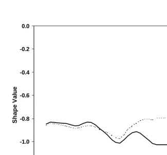
λ

are shown in Figure 6. In the figure, we added the graph of estimated

λ

for the model without empirical adjustment in a broken line to see effect of the adjustment. Its values after 1960 are fixed at the level of 1960 again. Shape values of the non-adjustment model deviate from that of the adjusted particularly in later cohorts with earlier truncation of the marriage process, tending to be larger which implies a more symmetric shape.

Notes: Solid line: Estimates with empirical adjustment, Broken line: Estimates without empirical adjustment.

Figure 6: Trends of Estimated Value of Parameter

λ

(Shape Value): Japanese

Female Cohorts born in 1933-70

-1.4 -1.2 -1.0 -0.8 -0.6 -0.4 -0.2 0.0

1930 1935 1940 1945 1950 1955 1960 1965 1970 1975 Cohort (Year of Birth)

S

h

ap

e V

a

lu

Figure 7: Observed and Predicted Age Specific First Marriage Rate: Japanese Female Cohort born in 1970

0.00 0.02 0.04 0.06 0.08 0.10

15 20 25 30 35 40 45 50

Age

Ra

te

Cohort born in 1970

● Observed

The results of estimation for the mean and the mode of age at first marriage, and the proportion never married at age 50 (γ) are portrayed (solid lines) in Figure 8a and -b along with estimates for the non-adjustment model (-broken lines) again. The trends show a smooth continuous transition from cohort to cohort except the relatively large fluctuation in C for cohorts born at the end of the World War II, probably caused by a flaw in raw statistics. For these indices, the original GLG model without adjustment yields similar estimates to those from the adjusted model for older cohorts. But the results from the former show somewhat different paths from the latter for younger truncated cohorts. These are expected from differences in the abilities of the models to trace age schedules of first marriage (see Figure 3, for instance).

What are the findings from the estimated trends of lifetime measures of first marriage by the empirically adjusted GLG model? The results for cohorts born in 1935-1970 indicate that there are five phases of behavioral change, of which the last three are relevant to the recent unprecedented nuptiality and fertility decline. The change was initiated with a delay in marriage by the cohort born in 1952, followed by a diffusion of never-marrying in cohorts born after 1959 along with prolonged delaying. Then there is an emerging new phase in which the timing shift of marriage is gradually ending in cohorts born after 1965, while the diffusion of never-marrying is rather accelerated. Close examination of hazard rates revealed that the diffusion of never-marrying in the second phase is related to the delaying behavior since marriage propensity in later ages seems to have a bound on increase, and some of postponed marriage have been foregone. On the contrary the diffusion of never-marrying in the third phase is caused by a decline in the propensity to marry even in higher ages as well as early ages. The results suggest that a new phase of marriage behavior is emerging among Japanese women born in and after 1965, which will result in steep increase in lifetime proportion never-marrying (Kaneko 2002).

Note that observation of the trends over cohorts born in from 1952 to 1970 is possible only via the application of some model, and a high level of accuracy in model is required to draw substantive conclusion. The original GLG model (CM model) seems not sufficient in the Japanese case for the recent period described above.

5.2 Application for Fertility Projection

Note: Solid line : Estimates with empirical adjustment Broken line : Estimates without empirical adjustment

Figure 8: Trends of Estimated and Projected Lifetime Measures of First Marriage:

Japanese Female Cohorts born in 1933-70

0 5 10 15 20 25

1930 1935 1940 1945 1950 1955 1960 1965 1970 1975

Cohort (Year of Birth)

P

ro

por

ti

on Ne

v

e

r M

a

rr

y

in

g

b. Trend of Estimated and Projected Value of Proportion Never Married at Age 50 (%) 22

23 24 25 26 27 28

1930 1935 1940 1945 1950 1955 1960 1965 1970 1975

Cohort (Year of Birth)

L

o

ca

ti

o

n

(

Y

ear

)

in this paper (Note 11). We briefly illustrate an immediate application of the GLG model to fertility in a system of fertility projection, following Kaneko (1993).

Let

F x C

_n

( ;

_n

, )

θ

be a function of age specific cumulative fertility rate of the n-th child at age x with proportion eventually having n-th child

C

_n and a set of other parameters

θ

_n, then:

( ;

,

θ

)

=

( ;

θ

)

n n n n n

F x C

C G x

(25)

where

G

denotes the distribution function of the GLG distribution. The function of age specific fertility rate of the n-th birth

f x C

_n

( ;

_n

,

θ

_n

)

is given by:

( ;

,

)

( ;

,

θ

)

=

n n

θ

n

=

( ;

θ

)

n n n n n

dF x C

f x C

C g x

dx

(26)

where g denotes PDF of the GLG distribution. However, the observed age specific fertility rate in completed age

a

should be given by

F a

_n

(

+ −

1)

F a

_n

( )

.

The estimation scheme is also identical to that for first marriages except substituting observed frequencies of n-th birth for those of first marriages. If schedules for all birth order are estimated, then the overall age specific cumulative birth rate F(x) is given simply by summing them up to the highest birth order as:

1

( )

( ;

,

)

=

=

å

L n n

θ

n n

F x

F x C

(27)

where L denotes the highest birth order. In practice, the class of highest birth order may include certain order of births (e.g. 5-th birth) and higher together so that the summation in (27) includes all births.

The model (27) contains

4

×

L

parameters, which seem to be many more than required to describe overall fertility schedules. Parameters for subsequent birth orders should be correlated and the relationships might be modeled so that we could reduce the number of parameters for parsimony. However, the maximum precision is attained in the original form as long as fertility rate by birth order are available, which is mostly the case with national data.

The empirical adjustment technique employed for first marriage schedule developed in the previous section is applicable to the model of fertility as well. Kaneko (1993) examined the error pattern of the model for each birth order with regard to Japanese female cohorts, and presented the adjustment functions in table form (see Table A-2 in the Appendix).

We now provide an illustration of the application of the model to cohort fertility. In Figure 9, the observed and predicted age specific fertility rates by birth order for Japanese female cohorts born in 1955 with data up to age 35 are plotted together. The model schedules follow the observed rates quite well for all birth orders.

Note: Fifth and higher birth order is not shown

Figure 9: Observed (as of 1991) and projected Cohort Fertility Rates: Japanese

Female Cohort born in 1955 0.00 0.05 0.10 0.15 0.20 0.25

15 20 25 30 35 40 45 50

Age F e rt ilit y R a te

Marks : Observed

Lines : Projected

All Birth

All Birth Order

0.00 0.02 0.04 0.06 0.08 0.10 0.12

15 20 25 30 35 40 45 50

Age Fe rt ilit y R a te

Marks : Observed

Lines : Projected

First Birth

Second Birth

Third Birth

The model projects the schedule of this cohort beyond age 35 (the point after which data was not available) to conclude the processes. Applying this projection procedure to every relevant cohort with some assumptions of future fertility behavior for very young cohorts, we obtain a prediction of the period fertility schedule. Using fertility data of cohorts born in 1935-75, the period age specific fertility rates for the year 1985 through 1990 are reconstructed by the model system. The fits are visually presented in Figure 10, which indicates that the system is capable of generating period fertility schedules with adequate precision for most practical purposes (Note 12).

Figure 10: Observed and Projected Period Fertility Rates: Japanese Female,

1985, 1990

0.00 0.05 0.10 0.15 0.20

15 20 25 30 35 40 45 50

Age

F

e

rt

il

it

y

R

a

te

Marks : Observed

Lines : Projected

6. Summary and Conclusion

The first purpose of the present paper is to show that recognition that the Coale-McNeil (CM) nuptiality model is equivalent to the generalized log gamma (GLG) distribution model allows an expansion of possible application of the model. Some of these applications are illustrated. First, by taking advantage of single parameter representation for the shape of the GLG model, a simple method to derive a country specific standard schedule is proposed. In this course, the significance of the shape specific to a country or region, represented by single value by the GLG model, is indicated. Second, we demonstrated a regression analysis of the effects of covariates on marriage timing. Immediate application of the theories, techniques and software packages of the GLG statistical model to analyze first marriage is main advantage of the new recognition. Here the effects of individual characteristics on first marriage timing were measured with the GLG regression technique, taking account of types of marriage, such as arranged and non-arranged marriages, with the competing risk framework. In our illustration of analysis on Japanese female experiences, we found interesting hidden effects of covariates that would not be found otherwise. These applications revealed also some mechanisms that determine the shape of distribution underlying the first marriage schedule. Heterogeneities of the marriage processes depending both on individual characters and types of marriage (presence of arranged marriage) in Japanese case promote symmetry in shape, which is significantly different from the shape of the Coale-McNeil global standard derived from Swedish experiences. When both types of heterogeneity are controlled, the shape of the schedule of each underlying process tends to follow the global standard.

It should be noted that every aspect of arguments on the GLG model for the first marriage schedule can be directly applied for the fertility schedule by birth order, because of the formal equivalence in structures of those processes. Finally, we demonstrated an application of the enhanced model to the fertility projection system. The performance of the system to predict cohort and period age specific fertility rates seems satisfactory so that it is utilized for country specific precise fertility projection.

7. Acknowledgements

Notes

1. This may be regarded as a continuous version of the age specific first marriage rate that is in the strict sense defined by a definite integral of

f x

( )

over the relevant age range.

2. Pearson's correlation coefficient between meeting and waiting time to first marriage is -0.48 (that of meeting and time to engagement is -0.45, and of meeting and engagement period is -0.22) for Japanese women born in 1938-54. Partial correlation coefficient between the age at meeting and the waiting time to first marriage with cohort effect controlled is virtually not affected (-0.45). The analysis was carried out on the data from the Ninth National Fertility Survey in 1987 conducted by National Institute of Population and Social Security Research. 3. PDF of the Gamma distribution with two parameters,

k

and

δ

, is:

[ ]

1

(

)

( )

exp

0

( )

−

=

−

>

Γ

k

t

f t

t

t

k

δ δ

_δ

while that of the GG distribution with

additional parameter,

η

, is;

1

(

)

( )

exp

(

)

0

( )

−

é

ù

=

_ë

−

_û

>

Γ

k

t

f t

t

t

k

η

η

δη δ

_δ

4. The gamma function and the incomplete gamma function are here defined as:

1 0

( )

∞ − −

Γ

=

_ò

y u

y

u

e du

and 1

0

1

( , )

( )

− −

=

Γ

ò

t y u

I y t

u

e du

y

) respectively.

5.

k

is corresponding to

α β

in equation (1).

6. Some of statistical packages include regression application with the generalized gamma distribution. We here utilized LIFEREG procedure in SAS/STAT. Constant term of u, b, and

λ

are respectively correspond to INTECEPT, SCALE, and SHAPE in the SAS output of the procedure with option NOLOG.