Design and Evaluation of a Hierarchical Control Algorithm for an Electric Active Stabilizer Bar System

(1)

*Corresponding Author’s Address: Nanjing University of Science & Technology, Department of Mechanical Engineering, ₅₆₅

0 INTRODUCTION

Vehicle roll motion can reduce the roll stability and handling stability. Improving the vehicle roll dynamics response is important. Previously, the passive stabilizer bar was installed to stabilize the vehicle body, but the performance is limited. Thus, some active roll control (ARC) systems have been developed. One of the effective solutions is active stabilizer bar (ASB) system. ASB system can generate active anti-roll torque in real time, reduce the body roll angle and roll rate, and it is suitable for applying to the mass production of cars because of the low cost and simple structure.

Therefore, many researchers have been focusing on ASB systems. The HIL benches for hydraulic ASB are designed and tested in [1] to [3]. An electric active stabilizer suspension system is developed to control vehicle roll motion. The actual vehicle tests proved superior roll stability and ride comfort in [4] to [6]. A control logic for the ASB system with rotary-type

hydraulic stabilizer actuators is proposed in [7]. The

control logic consists of a feedforward controller and a feedback controller. Through the test, the ASB system demonstrated the successful reduction of the

roll motion under all conditions. Moreover, [8] puts

forward a linear quadratic (LQ) controller based on two-level architecture.

There has also been some research on coordination control of ASB and other chassis control

systems. Yim et al. [9] present a method for designing

a controller that uses ASB and ESP for rollover prevention. Moreover, an integrated control strategy of the differential braking, the semi-active suspension

damper and the active roll moment is analysed in [10].

In this paper, a novel hierarchical control scheme of ASB is put forward. The upper-level controller calculates active anti-roll torque. The middle-level controller distributes active anti-roll torque between front and rear active stabilizer bars. The lower level controller is employed to control the output torque of actuators. The structure of this paper is as follows. The system dynamic models including vehicle and tire model, road input model and ASB actuator model are presented in Section 1. The hierarchical controller of the ASB system is designed in Section 2. In Section 3, numerical simulations and HIL experiments are implemented, together with results. Finally, the conclusions of the paper are summarized in Section 4.

1 SYSTEM DYNAMIC MODELS

1.1 Vehicle and Tire Model

A 14 degree-of-freedom (DOF) vehicle dynamics

model is adopted in this paper [11], which includes

the longitudinal, lateral, roll, yaw, pitch, vertical and

Design and Evaluation of a Hierarchical Control Algorithm

for an Electric Active Stabilizer Bar System

Kong, Z. - Pi, D. - Wang, X. - Wang, H. - Chen, S.

Zhenxing Kong - Dawei Pi*_{- Xianhui Wang - Hongliang Wang - Shan Chen}

Nanjing University of Science & Technology, Department of Mechanical Engineering, China

This paper describes a novel hierarchical control algorithm for the electric active stabilizer bar (ASB) system, which is applied to a four-wheeled road vehicle. The proposed control algorithm is designed to improve vehicle roll and yaw dynamics. The upper-level controller calculates the target active anti-roll torque via sliding mode control, which is aimed at improving the roll stability. The middle-level controller distributes active anti-roll torque between front and rear axle via fuzzy control, which can improve the handling stability through changing lateral load transfer of front and rear axles in real time. The lower level controller is employed to control the output torque of ASB actuators via PI control and improve the output characteristic of actuators with excellent response and stability. The numerical simulation and hardware-in-the-loop (HIL) experiment are carried out to evaluate the performance of the proposed control algorithm. It is demonstrated that the ASB system based on proposed control algorithm makes a significant improvement in the vehicle roll stability, ride comfort and handling stability.

Keywords: active stabilizer bar, hierarchical control, electric, sliding mode control, fuzzy control, numerical simulation, hardware-in-the-loop experiment

Highlights

(2)

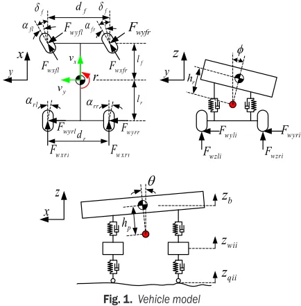
rotational motion of four wheels, vertical motion of the vehicle body. The top, front and left view of a vehicle system model is presented in Fig. 1. Moreover,

the Dugoff tire model [12] and [13] is adopted, which

can reflect the longitudinal tire force and lateral force variation with the slip ratio, the side slip angle, and the tire vertical load.

f

δ

fl

α

x y

fr

α

rl

α α_rr

r

y v

x

v z

y

φ

f

δ

w xrr F w xrl F wxfl

F Fwxfr

w yrr F

wzri F wyrl

F wyfl

F Fwyfr

wzli F

wyri F wyli

F

f

l

r d

r

l

r h

f d

z

x

θ

b

z

wii

z

qii

z p

h

Fig. 1. Vehicle model 1.2 Road Input Model

The road roughness plays a major role in the motion of the vehicle. Considering the road roughness of four wheels, a C-level road model is established based on the filtered white noise method in MATLAB/Simulink

[14].

1.3 ASB Actuator Model

The electric ASB actuator consists of left-half and right-half stabilizer bars, a brushless direct current (BLDC) motor, a reduction gear, a housing and two

bushings [6]. The force diagram of an active stabilizer

bar is presented in Fig. 2.

b

2/

t

bar

F Fbar

ARC M

φ

MActuator

Fig. 2. Force diagram of an electric active stabilizer bar

The relationship between MActuator and MARC is

denoted by Eqs. (1) and (2).

F M

t M

b

bar= ARC = Actuator, (1)

M t

bM

ARC = Actuator. (2)

Therefore, the output torque of ASB actuators can be calculated by Eq. (3) and (4).

M t

b M

ARC f f

f Actuator f

, = , , (3)

M t

b M

ARC r r

r Actuator r

, = , , (4)

where MActuator,i is the output torque of ith ASB

actuator, MARC,i is the active anti-roll torque of ith ASB

system; t is the length of the stabilizer bar, and b is length of the lever.

To calculate and debug easily, the BLDC motor model is replaced by the direction current (DC) motor model [15] by Eqs. (5) to (8).

U U L M dI

dt IR

e

− =

(

−

)

+ , (5)

Ue=Keω, (6)

T T J d

dt B

e− =l +

ω _ω_,₍₇₎

Te=K It . (8)

Considering the reduction gear, the output torque of front and rear ASB actuators are given by Eqs. (9) and (10).

MActuator f, =iTe f, , (9)

MActuator r, =iTe r,, (10)

where Ke is back-emf constant, Kt torque constant,

i transmission ratio of the reduction gear, I motor

current, B motor damping coefficient, J motor inertia,

M electromotive damping, R armature resistance,

Te electromagnetic torque, Tl load torque, U supply

voltage of the armature, Ue back electromotive force

(emf), and ω motor angular velocity.

2 HIERARCHICAL CONTROLLER DESIGN

(3)

hierarchical control system includes three level controllers:

1. Upper-level controller: to improve the roll stability of vehicles, the upper-level controller is designed to generate the target active anti-roll torque.

2. Middle-level controller: the middle-level controller is designed to distribute the active anti-roll torque between front and rear active stabilizer bars, which can improve yaw stability.

3. Lower level controller: to improve the output performance of the ASB actuator, the lower level controllers are designed to control the output torque of the ASB actuator.

Middle Level Controller Upper Level

Controller

r

a

v

x y

f

,

φ

,

δ

ARC M

Lower Level Controller 1

Lower Level Controller 2

Front ASB

Rear ASB

14 DOF Vehicle Model

f

δ

q

Steering Input Road Disturbances Control Algorithm

f ARC

M ,

r ARC

M ,

Fig. 3. Block diagram of the control system

Sliding Mode Controller Roll Angle

Reference Model

y

a

φ

_t

φ

ARC

M

+

-Fig. 4. Diagram of upper level controller

0 1 2 3 4 5 6 7 8 9 10

0 1 2 3 4 5 6

Lateral acceleration [m/s2]

Ro

ll a

ng

le

[d

eg]

Vehicle with passive stabilizer bar Vehicle with active stabilizer bar

Fig. 5. Roll angle reference model

2.1 Upper-Level Controller

The upper-level controller is designed based on the sliding mode control theory to control the roll angle, which can generate the target active anti-roll torque. The diagram of the upper-level controller is shown in Fig. 4.

The roll reference model [4] shown in Fig. 5 is

adopted to generate the target roll angle. In comparison with the vehicle equipped with passive stabilizer bars, the vehicle equipped with electric stabilizer bar has smaller roll angle at the same lateral acceleration, which means better roll stability.

The vehicle roll dynamic model [6] is presented

by Eq. (11).

φ φ φ

φ φ φ φ

=

(

)

+

( )

+

( )

=

(

)

+

(

)

+

( )

f t b t M d t

f t f t b t M

ARC

A

, ,

, , ∆ , , _RRC+d t

( )

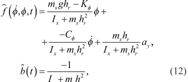
, (11)

The parameters of the vehicle roll dynamic model are estimated as (Eq. (12)):

f t m gh K

I m h

C

I m h

m h

I m h a

s r

x s r

s r

x s r y

φ φ φ

φ φ

φ , ,

(

)

= −

+ +

+ −

+ + +

2

2 2 ,,

,

b t

Ix m hs r

_{( )}

₌ − +

1

2 (12)

where ms is sprung mass, ay lateral acceleration, Kϕ

total suspension roll stiffness, Cϕ total suspension

roll damping, g acceleration of gravity, hr distance

between roll axis and centre of gravity, Ix roll moment

of inertia and ϕ roll angle.

Define the error between target roll angle ϕt and

actual roll angle ϕ as (Eq. (13)):

e= −φ φt . (13)

To reduce static error of the system, define the integral sliding surface as (Eq. (14)):

s c edt c e e c c= 1

_∫

+ 2 +,

(

1, 2 >0

)

, (14)

then

s c e c e e

c e c e f t f t

b t M_ARC

= + + =

= + −

(

)

−

(

)

−

( )

1 2

1 2 φ φ, , ∆ φ φ, ,

−−d t

( )

+φ_t. (15)

The uncertainty of the system is given by Eq. (16).

(4)

Choose the reaching condition which guarantees the asymptotic rapidity and stability as follows Eq. (17):



s= −εsgn( )s Ks− ,

(

ε,K>0

)

. (17)

The gains are determined as (Eq. (18)):

ε= + +F D η,K>0. (18)

The control law is designed as follows:

M

b t

c e c e f t

s Ks ARC=

_{( )}

+ −

(

)

+ +        

1 1 2

φ φ ε

, ,

sgn( )

. (19)

Consider a Lyapunov function candidate in Eq. (20):

V=1s 2

2

. (20)

The sliding condition is satisfied according to Eq. (21):

V ss s c e c e f t f t

b t M_ARC d t

= = + −

(

)

+

(

)

−

( )

−

( )

+

[ ₁ ₂ ϕ ϕ, , ∆ φ φ, ,

φ φ φ φ ε ε t t

s f t d t s Ks

s F D s

]

, , sgn( )

sgn( = = −_

(

)

−

( )

+ − − _{ ≤} ≤ + − ∆ )) ( ) ( ) . −

[

]

= = + − − ≤ ≤ + − − = − − ≤ Ks

F D s s Ks

F D s s Ks s Ks

ε

ε η

2

2 2

0 (21)

To eliminate the high-frequency chatter further, the sign function is replaced by a saturation function in Eq. (22):

sat s s s s s Φ Φ Φ Φ    _ = ≤

( )

>

      1 1 sgn

, (22)

where Φ is boundary-layer thickness.

The output of sliding mode controller is presented by Eq. (23):

M

b t c e c e f t

s _Ks ARC=

( )

 + −

(

)

+ +   1 1 2

φ φ, , εsat(Φ) , (23)

that is

M m gh K C m h a

I m h c e c e s

ARC s r s r y

x s r

= − − + − − + + + + ( ) ( ) ( ) φ φ φφ ε   2

1 2 sat

Φ KKs 



 . (24)

Thus the control law obtained above can meet the requirement of system stability and track the target

value accurately. All control parameters are listed in Table 1.

Table 1. Controller parameters

c1 = 140 K = 10 Φ = 0.1

c2 = 10 ε = 0.1

2.2 Middle Level Controller

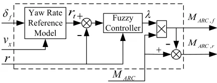
The middle-level controller is designed to distribute the anti-roll torque between front and rear active stabilizer bars. Moreover, the good coordination of roll stability and yaw stability can be guaranteed [18]. The diagram is shown in Fig. 6.

Fuzzy

Controller MARC,f

r ARC M , t

r

λ

ARC M Yaw Rate Reference Model f

δ

x

v

−

+

−

Fig. 6. Diagram of middle-level controller

Based on two DOF linear vehicle model [9], the

steady-state value of target yaw rate rt,ss is achieved as

follows (Eq. (25)):

r v l

mv l l C l C

t ss x

x f r r f f , / , = +  −   _ 1 2 2

δ (25)

where vx is longitudinal velocity, δf front wheel angle, Cf / Cr cornering stiffness of front/ rear axle, l wheel

base, and lf / lr front/ rear share of wheel base.

Moreover, the yaw rate transient response is characterized in Eq. (26).

r

s r

t1 t ss

1

0 1 1

= +

. , . (26)

Considering limitation of the road friction, the limited value of yaw rate [17] is given as:

r g v t x 2 0 85

= . µ , (27)

where μ is road friction coefficient.

Thus, the target yaw rate is computed as follows (Eq. (28)):

rt =sgn

( )

rt1 ⋅min

(

r rt1, t2

)

. (28)

The inputs of the fuzzy controller are yaw rate r

(5)

controller is the distribution coefficient λ

(λ =MARC f, MARC∈

[ ]

0 1, ).

In the fuzzification step, linguistic variables are

used to make the input variables r and dr and the

output variable λ compatible with the condition of

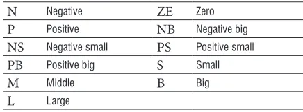
the knowledge-based rules. The linguistic terms are shown in Table 2. The fuzzy sets used for inputs and outputs are defined as:

{r}={N, ZE, P}

{dr}={NB, NS, ZE, PS, PB}

{λ}={ZE, S, M, B, L}.

Table 2. Linguistic terms for middle-level controller

N Negative _ZE Zero

P Positive _NB Negative big NS Negative small PS Positive small PB Positive big _S Small

M Middle B Big

L Large

During the fuzzy decision process, a list of fuzzy rules is defined on the basis of expert knowledge and extent simulation. The Mamdani fuzzy inference system is adopted, and the weights of the rules are considered to be 1. The fuzzy rules are shown in Table 3. These rules are introduced on the basis of the following criteria.

Table 3. Fuzzy rules for middle level controller

r dr λ r dr λ

N NB ZE ZE PS M

N NS S ZE PB M

N ZE M P NB L

N PS B P NS B

N PB L P ZE M

ZE NB M P PS S

ZE NS M P PB ZE

ZE ZE M

Criterion 1: if r is NB and dr is N, then λ is ZE. In this case, the vehicle is in a serious understeer state. The lateral load transfer of front axle is set to increase, and the lateral load transfer of rear axle is set to decrease. Thus, the distribution coefficient tends to zero.

Criterion 2: if r is PB and dr is N, then λ is L. In this case, the vehicle is in a serious oversteer state. The lateral load transfer of front axle is set to decrease, and the lateral load transfer of rear axle is set to increase. Thus, the distribution coefficient tends to be large.

Criterion 3: if r is ZE or dr is ZE, then λ is M. In this case, the vehicle is in a stable state. The lateral load transfer of the front axle is set to be a little smaller than the lateral load transfer of the rear axle, which can make the vehicle be in a slight understeer state. Thus, the distribution coefficient is set about 0.55.

The centre-of-area defuzzification method is used to scale and map the fuzzy output to produce an output value for the control system. Through many

simulations and analyses, r is set within the range of

[–1 rad, 1 rad], dr is set within the range of [–0.25

rad/s, 0.25 rad/s], and λ is set within the range of [0,

1]. The membership functions of input and output variables are shown in Fig. 7.

a)

-1 -0.75 -0.5 -0.25 0 0.25 0.5 0.75 1

0 0.2 0.4 0.6 0.8 1

r [rad/s]

De

gr

ee

o

f m

em

be

rs

hi

p N ZE P

b)

-0.2 -0.1 0 0.1 0.2

0 0.2 0.4 0.6 0.8 1

dr [rad/s]

De

gr

ee

o

f m

em

be

rs

hi

p NB NSZEPS PB

c) 0 0.2 0.4 0.6 0.8 1

0 0.2 0.4 0.6 0.8 1

λ

De

gr

ee

o

f m

em

be

rs

hi

p

B

S L

ZE M

(6)

Therefore, active anti-roll torques of the front and rear active stabilizer bars are given by Eq. (29) and (30).

MARC f, =λMARC, (29) MARC r, = −

(

1 λ

)

MARC. (30)

2.3 Lower Level Controller

The lower level controller is designed with PI control theory to control the output torques of the front and rear active stabilizer bars, which can improve the actuator output performance with excellent response and stability. In practical engineering application, the control of actuator output torque can be realized by

controlling the electric current of motors [16]. The

control diagram of the system is shown in Fig. 8.

PI

Controller CircuitDrive DC Motor Model

I

t

I

α

l T

e

T

−

+

Fig. 8. Diagram of lower level controller

Considering the ASB actuator model in section 1.3, the target electric current of motors can be presented in Eq. (31) and (32).

I b

iK t M

t f f

t f ARC f

, = , , (31)

I b

iK t M

t r r

t r ARC r

, = , . (32)

The input of PI controller is the current error ei

(ei = It – I), and the output of PI controller is PWM duty ratio α of the motor current. The control algorithm is given by Eq. (33). The controller parameters are listed in Table 4.

α =k e k e dt_{p i}+ _i

∫

_i . (33)

Table 4. Controller parameters

kp = 0.1 ki = 40

3 SIMULATION AND EXPERIMENT

3.1 Numerical Simulation

The numerical simulation is carried out to evaluate the performance of the ASB system under typical

manoeuvres. The parameters of vehicle and ASB actuator adopted are listed in Tables 5 and 6.

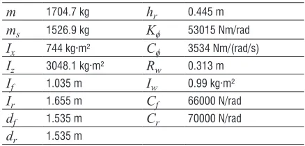
Table 5. Parameters of the vehicle

m 1704.7 kg h_r 0.445 m ms 1526.9 kg Kϕ 53015 Nm/rad Ix 744 kg·m² Cϕ 3534 Nm/(rad/s) Iz 3048.1 kg·m² Rw 0.313 m If 1.035 m Iw 0.99 kg·m² Ir 1.655 m Cf 66000 N/rad df 1.535 m Cr 70000 N/rad dr 1.535 m

Table 6. The output characteristic of the actuator

Actuator Maximum torque Maximum torque rate ASB actuator 700 Nm 1600 Nm/s

The vehicle is set to travel on the C-level road with an initial speed of 80 km/h, no braking, and accelerating. The road friction coefficient µ is 0.8. The C-level road height is presented in Fig. 9.

Simulations are conducted with different types of suspensions, including ’without ASB’, ‘ASB without dynamic distribution’ (distribution coefficient

λ is 0.55) and ‘ASB with dynamic distribution’

respectively, under J-turn, sine wave and zero input manoeuvres. The front wheel angle under different manoeuvres above is shown in Fig. 10.

0 1 2 3 4 5 6 7 8 9 10

-0.02 -0.01 0 0.01 0.02

Time [s]

Ro

ad h

ei

gh

t [

m

]

Front left wheel Front right wheel Rear left wheel Rear right wheel

Fig. 9. The C-level road height of four wheels

3.1.1 Roll Stability

(7)

case is reduced by 46.1 % and 45.2 % in average. The roll angle is very close to target roll angle, which guarantees a rapid response and small static error.

Under sine wave manoeuvre, the roll angle follows the target value rapidly, even though the steering wheel input frequency reaches 0.7 Hz as shown in Fig. 12a. It is confirmed that the roll angle control of ASB system shows excellent frequency response characteristics.

a)

0 1 2 3 4 5 6 7 8 9 10

-3 -2 -1 0 1 2 3 4

Time [s]

Ro

ll a

ng

le

[d

eg]

Target value Without ASB

ASB with dynamic distribution

b)

0 1 2 3 4 5 6 7 8 9 10

-15 -10 -5 0 5 10 15

Time [s]

Ro

ll r

at

e [

de

g/

s]

Without ASB

Fig. 12. Roll motion under sine wave manoeuvre; a) roll angle and b) roll rate

Figs. 13a and b show vehicle roll motion under zero input manoeuvre. The roll angle and roll rate caused by the road input excitation both decreases. Considering the human body sensitivity to roll vibration (around 0.8 Hz) and roll resonant frequency (around 2 Hz), the PSD of roll rate in the 0.3 Hz to 3 Hz domain is used to evaluate the vehicle ride

comfort [5]. From Fig. 13c, the PSD of roll rate in the

frequency range of 0.3 Hz to 3 Hz is reduced by 5 dB to 20 dB. Obviously, the vehicle with the ASB system has great ride comfort performance.

a) 0 1 2 3 4 5 6 7 8 9 10

0 0.05 0.1 0.15 0.2

Time [s]

Fr

on

t whe

el

a

ng

le

[r

ad

]

b) 0 1 2 3 4 5 6 7 8 9 10

-0.2 -0.1 0 0.1 0.2

Time [s]

Fr

on

t whe

el

a

ng

le

[r

ad

]

Fig. 10. Front wheel angle under different manoeuvres; a) J-turn and b) sine wave

a) 0 1 2 3 4 5 6 7 8 9 10

-0.5 0 0.5 1 1.5 2 2.5 3 3.5 4

Time [s]

Ro

ll a

ng

le

[d

eg]

b) 0 1 2 3 4 5 6 7 8 9 10

-5 0 5 10

Time [s]

Ro

ll r

at

e [

de

g/

s]

Without ASB

(8)

a) 0 1 2 3 4 5 6 7 8 9 10

-0.4 -0.3 -0.2 -0.1 0 0.1 0.2 0.3

Time [s]

Ro

ll a

ng

le

[d

eg]

Witout ASB

b)

0 1 2 3 4 5 6 7 8 9 10

-3 -2 -1 0 1 2

Time [s]

Ro

ll r

at

e [

de

g/

s]

Without ASB

c) 10

0 ₁₀1

-80 -60 -40 -20 0 20

Frenquency [Hz]

PS

D o

f r

ol

l r

at

e [

dB

/Hz

]

Without ASB

Fig. 13. Roll motion under zero input manoeuvre; a) roll angle, b) roll rate and c) PSD of roll rate

3.1.2 Handling Stability

The simulation results of yaw rate are shown in Fig. 14. Compared with the ‘without ASB’ case, the yaw rate is closer to the target value in the ‘ASB without dynamic distribution’ and ‘ASB with dynamic distribution’ cases. Moreover, the yaw rate peak values of two cases are both reduced.

Under the J-turn manoeuvre, the yaw rate of ‘ASB with dynamic distribution’ case has better transient and steady-state response characteristics in comparison to ‘ASB without dynamic distribution’ case, which indicates smaller overshot and oscillation of yaw rate. Moreover, yaw rate of ‘ASB with dynamic distribution’ case is closer to the target value as shown in Fig. 14a.

a)

0 1 2 3 4 5 6 7 8 9 10

-10 -5 0 5 10 15 20 25 30

Time [s]

Ya

w r

at

e [

de

g/

s]

ASB without dynamic distribution ASB with dynamic distribution

b) 0 1 2 3 4 5 6 7 8 9 10

-40 -20 0 20 40 60

Time [s]

Ya

w r

at

e [

de

g/

s]

Fig. 14. Yaw rate under different manoeuvres; a) J-turn and b) sine wave

However, in Fig. 14b, the ‘ASB with dynamic distribution’ case has no significant effect on the yaw rate control in comparison to the ‘ASB without dynamic distribution’ case. Two important reasons are supposed as follows:

1. Under extreme steering manoeuvres, the vehicle is in a serious unstable state. Considering the limitation of the coupling relationship between roll and yaw dynamics, it is very difficult to implement the vehicle yaw rate control.

(9)

the high-frequency region due to the limitation of the ASB actuator’s output characteristic, such as the torque rate.

In general, the ASB system with dynamic distribution provides a more rapid response and smaller oscillation of the yaw rate, which considerably improves vehicle handling stability.

3.2 Hardware-in-the-loop Experiment

The experiments are performed based on an HIL system. The HIL system includes the real-time simulation system (AutoBox), ASB electric control unit (ASB ECU), ASB actuators and force sensors. Fig. 15 shows the block diagram of the HIL system. The AutoBox runs a vehicle dynamics model, a Dugoff tire model, and a road input model, and exports vehicle state signals. According to those signals, ASB control algorithm in ASB ECU calculates the target anti-roll torque of front and rear ASB actuator. ASB actuators generate actual anti-roll torque, which is measured by force sensors. The actual anti-roll torque of front and rear ASB actuator are imported to the vehicle dynamics model.

Vehicle Dynamics

Model

Dugoff Tire Model ASB ECU

(ASB Control Algorithm)

Front ASB Actuator Vehicle State

Target Anti-roll Torque_front

Actual Anti-roll Torque_front

Rear ASB Actuator Target Anti-roll

Torque_rear

Actual Anti-roll Torque_rear AutoBox

Road Input Model

Fig. 15. Block diagram of HIL system

The initial setup of the experimental vehicle is the same as that in numerical simulation (Section 3.1). The HIL experiments are conducted under J-turn, sine wave, and zero input manoeuvres.

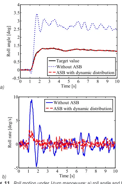
3.2.1 Roll Stability

Figs. 16 and 17 show the vehicle roll motion under J-turn and sine wave manoeuvre. The ‘ASB with dynamic distribution’ case reduces the vehicle roll angle and roll rate by 45.5% and 43.8%, respectively,

a) 0 1 2 3 4 5 6 7 8 9 10

-0.5 0 0.5 1 1.5 2 2.5 3 3.5 4

Time [s]

Ro

lla

ng

le

[d

eg

]

b)

0 1 2 3 4 5 6 7 8 9 10

-5 0 5 10

Time [s]

Ro

ll r

at

e [

de

g/

s]

Without ASB

Fig. 16. Roll motion under J-turn manoeuvre; a) roll angle and b) roll rate

a) 0 1 2 3 4 5 6 7 8 9 10

-2 0 2 4

Time [s]

Ro

ll a

ng

le

[d

eg]

b) 0 1 2 3 4 5 6 7 8 9 10

-15 -10 -5 0 5 10 15

Time [s]

Ro

ll r

at

e [

de

g/

s]

Without ASB

(10)

in average. Moreover, the roll angle follows the target value quickly with small chatter caused by the physical limitation of ASB actuators output characteristic. The steady-state error of roll angle is less than 0.2 deg. From Fig. 17a, the amplitude of roll angle is just about 0.15 deg bigger than the target value during the entire sine wave maneuver, and the phase of roll angle is the same as a target value, which means good frequency response characteristic of ASB system. It is verified that the proposed ASB control algorithm can improve the vehicle roll stability.

a)

0 1 2 3 4 5 6 7 8 9 10

-0.4 -0.3 -0.2 -0.1 0 0.1 0.2 0.3

Time [s]

Ro

ll a

ng

le

[d

eg]

Without ASB

b)

0 1 2 3 4 5 6 7 8 9 10

-3 -2 -1 0 1 2

Time [s]

Ro

ll r

at

e [

de

g/

s]

Without ASB

c)

100 101

-80 -60 -40 -20 0 20

Frequency [Hz]

PS

D o

f r

ol

l r

at

e [

dB

/Hz

] Without ASB_{ASB with dynamic distribution}

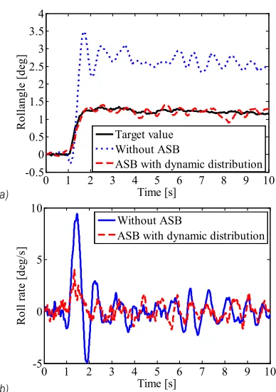
Fig. 18. Roll motion under zero input manoeuvre; a) roll angle, b) roll rate and c) PSD of roll rate

Fig. 18 shows vehicle roll response under zero input manoeuvre. From Fig. 18a and 18b, compared with ‘Without ASB’ case, ‘ASB with dynamic distribution’ reduces the roll angle and roll rate, which improves vehicle roll stability. From Fig. 18c, the PSD of roll rate decreases by 0 dB to -18 dB in the frequency range of 0.3 Hz to 3 Hz, which means better vehicle ride comfort.

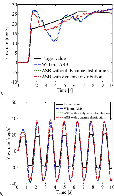
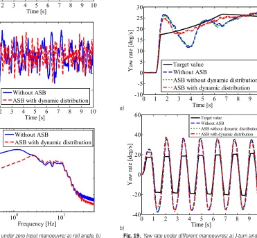
3.2.2 Handling Stability

Fig. 19 shows the vehicle yaw rate under J-turn and sine wave manoeuvre. ‘Without ASB’ and ‘ASB without dynamic distribution’ both have poor performance in vehicle yaw stability. From Fig. 19a, during 1 s to 2.5 s, the vehicle is in an oversteer state, and the anti-roll torque distribution reduces the overshot of yaw rate by 21.1%. During 2.5 s to 10 s, the anti-roll torque distribution reduces the oscillation of yaw rate, makes yaw rate follow the target value, and the steady-state error of yaw rate is less than 3 deg/s.

a)

0 1 2 3 4 5 6 7 8 9 10

-10 -5 0 5 10 15 20 25 30

Time [s]

Ya

w r

at

e [

de

g/

s]

b)

0 1 2 3 4 5 6 7 8 9 10

-40 -20 0 20 40 60

Time [s]

Ya

w r

at

e [

de

g/

s]

(11)

Thus, the vehicle is in a stable state. From Fig. 19b, since the limitation coupling relationship between the vehicle roll and yaw dynamics and physical limitation of ASB actuators output performance, the anti-roll torque distribution does not achieve desired control effect, which just slightly reduces the peak value of yaw rate by about 1deg/s in average. Above all, ASB system with dynamic distribution makes the vehicle yaw rate within a stable region and improves the vehicle handling stability under some extreme conditions.

4 CONCLUSIONS

A novel hierarchical control algorithm for an electric ASB system is proposed. Numerical simulations and HIL experiments are implemented to study the roll and handling stability of the vehicle with the proposed ASB control system under typical manoeuvres. Conclusions can be drawn as follows.

1. Three level controllers implemented for ASB system are devised based on the hierarchical control structure. In the upper level, a sliding mode controller is designed to generate active anti-roll torque, which improves vehicle roll stability. In the middle level, a fuzzy controller is proposed to distribute active torque between front and rear active stabilizer bars, which improves vehicle handling stability. In the lower level, a PI controller is applied to generate the actuator output torque.

2. Simulation and experimental results confirmed the reliability and precision of the ASB hierarchical control algorithm. The proposed control algorithm can reduce vehicle roll angle and roll rate effectively and improve vehicle yaw dynamics response.

In summary, the good coordination of the vehicle roll stability, ride comfort and handling stability can be achieved by the proposed ASB control algorithm.

5 ACKNOWLEDGEMENTS

This work was supported by the National Science Foundation (Grant No. 51205204, No. 51205209), the Fundamental Research Funds for the Central Universities (Grant No. 30915118832), and the Six Talent Program of Jiangsu Province (Grant No. 2014003).

6 NOMENCLATURES

ay lateral acceleration of the vehicle [m/s2]

Cf cornering stiffness of front axle [N/rad]

Cr cornering stiffness of rear axle [N/rad]

Cϕ total suspension roll damping [N/(rad/s)]

df front tread [m] dr rear tread [m]

Fwxii/Fwyii/Fwzii longitudinal, lateral and vertical

force of iith_{wheel [N]}

g acceleration of gravity [m/s2_]

hp distance between pitch axis and centre of gravity

[m]

hr distance between roll axis and centre of gravity

[m]

i transmission ratio of reduction gear [-]

I motor current [A]

Iw moment of inertia of wheel [kg·m2]

Ix roll moment of inertia [kg·m2]

Iz yaw moment of inertia [kg·m2]

J motor inertia [kg·m2_]

Ke back-emf constant [V]

Kt torque constant [Nm/A]

Kϕ total suspension roll stiffness [Nm/rad]

lf front share of wheel base [m]

lr rear share of wheel base [m]

m total mass [kg]

ms sprung mass [kg]

M electromotive damping [H]

MActuator, f output torque of front ASB actuator [Nm] MActuator, r output torque of rear ASB actuator [Nm] MARC, f active anti-roll torque of front ASB system

[Nm]

MARC, r active anti-roll torque of rear ASB system

[Nm]

r yaw rate [rad/s]

rt target yaw rate[rad/s] R armature resistance [Ω]

Rw rolling radius of wheel [m]

Te electromagnetic torque [Nm]

Tl load torque [Nm]

U supply voltage of the armature [V]

Ue back electromotive force (emf) [V]

vx longitudinal velocity of the vehicle [m/s]

vy lateral velocity of the vehicle [m/s]

Zb displacement of vehicle body [m]

Zqii road height of iith wheel [m] Zwii displacement of iith wheel [m]

δf steering angle of the front wheel [rad]

μ road friction coefficient[-]

ϕ roll angle [rad]

ϕt target roll angle [rad]

(12)

7 REFERENCES

[1] Sorniottia, A., Morgandoa, A., Velardocchiaa, M. (2006). Active roll control: system design and hardware-in-the-loop test bench. Vehicle System Dynamics: International Journal of Vehicle Mechanics and Mobility, vol. 44, suppl. 1, p. 489-505,

DOI:10.1080/00423110600874677.

[2] Cimba, D., Wagner, J., Baviskar, A. (2006). Investigation of active torsion bar actuator configurations to reduce vehicle body roll. Vehicle System Dynamics: International Journal of Vehicle Mechanics and Mobility, vol. 44, no. 9, p. 719-736,

DOI:10.1080/00423110600618280.

[3] Sorniotti, A., D’Alfio, N. (2007). Vehicle dynamics simulation to develop an active roll control system. SAE Technical Paper, no. 2007-01-0828, DOI:10.4271/2007-01-0828.

[4] Buma, S., Ookuma, Y., Taneda, A., Suzuki, K., Cho, J.-S., Kobayashi, M. (2010). Design and development of electric active stabilizer suspension system. Journal of System Design & Dynamics, vol. 4, no. 1, p. 61-76, DOI:10.1299/jsdd.4.61.

[5] Mizuta, Y., Suzumura, M., Matsumoto, S. (2010). Ride comfort enhancement and energy efficiency using electric active stabiliser system. Vehicle System Dynamics: International Journal of Vehicle Mechanics & Mobility, vol. 48, no. 11, p. 1305-1323, DOI:10.1080/00423110903456909.

[6] Jeon, K., Hwang, H., Choi, S., Kim, J., Jang, K., Yi, K. (2012). Development of an electric active roll control (ARC) algorithm for a SUV. International Journal of Automotive Technology, vol. 13, no. 2, p. 247-253, DOI:10.1007/s12239-012-0021-8.

[7] Kim, S., Park, K., Song, H.J., Hwang, Y.K., Moon, S.J., Ahn, H.S., Tomizuka, M. (2012). Development of control logic for hydraulic active roll control system. International Journal of Automotive Technology, vol. 13, no. 1, p. 87-95, DOI:10.1007/ s12239-012-0008-5.

[8] Varga, B., Németh, B., Gáspár, P. (2015). Design of anti-roll bar systems based on hierarchical control. Strojniški vestnik - Journal of Mechanical Engineering, vol. 61, no. 6, p. 374-382,

DOI:10.5545/sv-jme.2014.2224.

[9] Yim, S., Jeon, K., Yi, K. (2012). An investigation into vehicle rollover prevention by coordinated control of active anti-roll

bar and electronic stability program. International Journal of Control, Automation, Systems, vol. 10, no. 2, p. 275-287,

DOI:10.1007/s12555-012-0208-9.

[10] Her, H., Suh, J., Yi, K. (2015). Integrated control of the differential braking, the suspension damping force and the active roll moment for improvement in the agility and the stability. Proceedings of the Institution of Mechanical Engineers, Part D: Journal of Automobile Engineering, vol. 229, no. 9, p. 1154-1154, DOI:10.1177/0954407014550502.

[11] Ghike, C., Shim, T. (2006). 14 degree-of-freedom vehicle model for roll dynamics study. SAE Technical Paper, no. 2006-01-1277, DOI:10.4271/2006-01-1277.

[12] Dugoff, H., Fancher, P.S., Segel, L. (1970). An analysis of tire traction properties and their influence on vehicle dynamic performance. SAE Technical Paper, no. 700377,

DOI:10.4271/700377.

[13] Guntur, R., Sankar, S. (1980). A friction circle for Dugoff’s tyre friction model. International Journal of Vehicle Design, vol. 1, no. 4, p. 373-377, DOI:10.1504/IJVD.1980.061234.

[14] Zhang, L.J., Zhang, T.X. (2008). Study on general model of random inputs of the vehicle with four wheels correlated in time domain. Transactions of the Chinese Society of Agricultural Machinery, vol. 27, no. 7, p. 75-78, DOI:10.3969/j. issn.1000-1298.2005.12.008.

[15] Zhang, H., Liu, J., Ren, J., Zhang, Y., Gao, Y. (2009). Research on electric power steering with BLDC drive system. IEEE 6th International IEEE Power Electronics and Motion Control Conference, p. 1065-1069, DOI:10.1109/ IPEMC.2009.5157543.

[16] Kim, J.-H., Song, J.B. (2002). Control logic for an electric power steering system using assist motor. Mechatronics, vol. 12, no. 3, p. 447-459, DOI:10.1016/S0957-4158(01)00004-6.

[17] Pi, D.-W., Chen, N., Zhang, B.-J. (2011). Experimental

demonstration of a vehicle stability control system in a split-μ

manoeuvre. Proceedings of the Institution of Mechanical Engineers, Part D: Journal of Automobile Engineering, vol. 225, no. 3, p. 305-317, DOI:10.1177/09544070JAUTO1541.