* Corresponding author: Tel: +985431132450 Email:[email protected]
Hydrodynamics of Sieve Tray Distillation Column Using
CFD Simulation
Mozhgan Movahedi Parizi and Rahbar Rahimi*
Department of Chemical Engineering, Shahid Nikbakht’s Faculty of Engineering, University of Sistan and Baluchestan, Sistan and Baluchestan, I. R. Iran
(Received 19 November 2014, Accepted 11 December 2015)
Abstract
Sieve trays are widely used in the gas- liquid contactors such as distillation and absorption towers. In this article, a three-dimensional, two phase CFD model using Euler-Euler framework was developed to simulate a distillation tower with two sieve trays. Hydrodynamic simulation of air and water system in different rates of gas phase was carried out and velocity distribution parameters, clear liquid height and froth height were calculated and compared to the experimental data and the literature simulation result. Liquid velocity distributions on the two trays were found to be in relatively good agreement with experimental data. It was found that heights of accumulated liquid in the down-comers are not equal.
Keywords:
CFD, Distillation, Hydrodynamics, Sieve Tray.1. Introduction
Distillation is the dominant separation process in the chemical and petroleum industries. One of the major factors that favor distillation is the fact that large diameter columns can be designed and built with confidence. Columns with sieve trays have been used in the chemical and petrochemical industry for their simplicity, low construction cost and low pressure drop [1, 2, 3]. Knowledge of tray hydraulics is necessary for the prediction of separation efficiency and overall tray performance. Tray efficiency depends on many involved interrelated parameters; one of them is the flow pattern of a gas-liquid mixture. Flow could follow either froth or spray regime [4]. In recent years, there are considerable academic and industrial interests in the use of computational fluid dynamics (CFD) model for describing the hydrodynamics of sieve trays [4, 5]. The important advantage of the CFD simulations is that the influence of tray geometry is automatically taken in to account by the CFD codes. Krishna et al. [6], and Van Baten and Krishna [7] developed a three-dimensional CFD model to study hydrodynamics of a circular sieve tray. The gas and liquid phases were treated as interpenetrating continuous phases and modeled within the Eulerian framework. Wang et al. [8] used a 3-D
pseudo-single-phases velocity and concentration on a distillation column tray and estimated an overall efficiency of 10-tray column. Fisher and Quarini [9] presented a 3-D transient model for vapor liquid hydrodynamics; they assumed a constant value of 0.44 for drag coefficient which is applicable for large bubbles. Gesit et al. [4], developed a 3-D CFD model to predict velocity distributions, clear-liquid height, froth height, and liquid holdup fraction in froth for various combinations of gas and liquid rates. Their study included only halve of the circular tray as the assumption of tray symmetry were made. Rahimi et al. [10] and Noriler et al. [11] further developed the CFD model to predict concentration and temperature distributions of rectangular and circular sieve trays. They focused on the development of reliable correlations for heat and mass transfer coefficients as well as reliable closure models. Malvin et al. [12], developed a 3-D CFD model based on the VOF-LES model to study the characteristics of the prevailing flow regimes in distillation sieve tray. They have concluded that the sphere equivalent diameter, ddrop,eq ,of a
Moreover, the previously mentioned CFD simulation models of sieve trays effectively focused on the hydraulic behavior of trays and did not include mass and heat transfer effects [10,11]. CFD simulation results can closely match experimental measurements as long as both are performed on the same model geometry. In this work, a CFD model has been developed to predict the flow patterns and hydraulics of a column having two sieve trays that uses air-water system. The complete experimental geometry, including whole sieve trays, inlet and outlet down-comers, were modeled based on the experimental work of Solari and Bell [13] sieve tray.
In order to resemble the experimental trays as closely as possible to the actual distillation tower, a gas distributor chamber under the lowest sieve tray included. Liquid velocity distributions, clear liquid height, froth height, dry pressure, average liquid and froth heights were reported and were compared with the available experimental results [13].
2.
Model equation
The numerical simulations presented are based on the two-fluid model in Eulerian-Eulerian approach because it gives better opportunities to study phase interactions and phase separation. In Eulerian- Eulerian point of view a volume control with fixed coordinates in fluid is considered. With the model focusing on the froth region of the sieve tray, the liquid and gas phases are taken to be the continuous and dispersed phases, respectively. Simulation used k-Ɛ two equations model for turbulent characteristics of froth region of tray. This model verified and used extensively [4, 6, 10, 14].
Modeling two phase flow requires the use of appropriate conservation equations that can account for the behavior of each of the phases and the interactions between them. The continuity equations for the gas and liquid phases are given by equations 1 and 2, respectively. Additional equations that
have taken the effects of phases interactions follow;
Continuity equation of the dispersed gas phase:
𝜕(𝑟𝐺𝜌𝐺)
𝜕𝑡 + ∇. 𝑟𝐺𝜌𝐺𝑉𝐺 = 0 (1)
Continuity equation of the continuous liquid phase:
𝜕 𝑟𝐿𝜌𝐿
𝜕𝑡 + ∇. 𝑟𝐿𝜌𝐿𝑉𝐿 = 0 (2)
Where, , r and V represent the density, volume fraction and velocity vector, respectively. The subscript letters of G and L are for the dispersed and the continuous phases, respectively.
2.1. Momentum equation
Conservation of gas and liquid phases momentums are given by equations 3 and 4, respectively. An accurate treatment of fluid momentum is important for several reasons. First, it is the only way to predict how fluid will flow through complicated geometry. Second, the dynamic forces (i.e., pressures) exerted by the fluid can only be computed from momentum considerations.
Gas phase:
𝜕
𝜕𝑡 𝑟𝐺𝜌𝐺𝑉𝐺 + ∇. 𝑟𝐺 𝜌𝐺𝑉𝐺𝑉𝐺 =
−𝑟𝐺∇𝑃𝐺 + ∇. 𝑟𝐺𝜇𝑒𝑓𝑓 ,𝐺 ∇𝑉𝐺+ ∇𝑉𝐺 𝑇 −
𝑀𝐺𝐿 (3)
Liquid phase:
𝜕
𝜕𝑡 𝑟𝐿𝜌𝐿𝑉𝐿 + ∇. 𝑟𝐿 𝜌𝐿𝑉𝐿𝑉𝐿 = −𝑟𝐿∇𝑃𝐿+ ∇. 𝑟𝐿𝜇𝑒𝑓𝑓 ,𝐿 ∇𝑉𝐿+ ∇𝑉𝐿 𝑇 + 𝑀𝐺𝐿 (4)
The gas and liquid volume fractions, 𝑟𝐺
and 𝑟𝐿, are related by the summation
Constraint as:
𝑟𝐺 + 𝑟𝐿 = 1 (5)
𝑃𝐺 = 𝑃𝐿 (6)
The effective viscosities of the gas and liquid phases are 𝜇𝑒𝑓𝑓 ,𝐺 and 𝜇𝑒𝑓𝑓 ,𝐿 , respectively.
μeff ,G = μlaminar ,G+ μturbulent ,G (7)
μeff ,L = μlaminar ,L+ μturbulent ,L (8)
The term MGL in the momentum equations represents interphase momentum transfer between the two phases. This will elaborate in section 2.2.
2.2. Closure models
Solution of continuity and momentum equations, equations 1 to 4, for velocities, pressure, and volume fractions require additional equations that relate the inter phase momentum transfer term, MGL, and the turbulent viscosities to the mean flow variables. The inter phase momentum transfer term, MGL, is basically inter phase drag force per unit volume. With the gas as the disperse phase, the equation for MGL is
𝑀𝐺𝐿 = 34𝐶𝐷
𝑑𝐺𝑟𝐺𝜌𝐿 𝑉𝐺 − 𝑉𝐿 𝑉𝐺 − 𝑉𝐿 (9)
Where 𝑉𝐺− 𝑉𝐿 is the relative velocity between the phases. 𝑑𝐺 is the Sauter mean
diameter of bubbles (equation 10), and 𝐶𝐷 is drag coefficient.
𝑑𝐺 = 𝑛𝑖𝑑𝑖
𝑛𝑖 (10)
The local Sauter mean diameter (𝑑𝐺) is required for using in Eq. 9.
As one can anticipate measurement of bubble size is not well accurate but, the procedure proposed by Krishna et al. [15] has resolved that obstacle. Drag coefficient𝐶𝐷, for the rise of a swarm of large bubbles in the churn turbulent regime is [15];
𝐶𝐷 = 43𝜌𝐿𝜌−𝜌𝐺
𝐿 𝑔𝑑𝐺
1
𝑉𝑠𝑙𝑖𝑝2 (11)
Where the slip velocity, 𝑉𝑠𝑙𝑖𝑝 = 𝑉𝐺− 𝑉𝐿 ,
is estimated from the gas superficial velocity, 𝑉𝑠. The average gas holdup fraction in the froth region is estimated as;
𝑉𝑠𝑙𝑖𝑝 =𝑟 𝑉𝑠
𝐺𝑎𝑣𝑒𝑟𝑎𝑔𝑒
(12)
Bennett et al.[16], correlation is used to estimate the average gas hold-up:
𝑟𝐺𝑎𝑣𝑒𝑟𝑎𝑔𝑒 =
1 − 𝑒𝑥𝑝 −12.55(𝑉𝑠 𝜌𝜌𝐺
𝐿−𝜌𝐺)
0.91 (13)
From the given equation the inter phase momentum transfer term as a function of local variables becomes [15]:
𝑀𝐺𝐿 = 𝑟𝐺
𝑎𝑣𝑒𝑟𝑎𝑔𝑒 2
1.0−𝑟𝐺𝑎𝑣𝑒𝑟𝑎𝑔𝑒 𝑉𝑠2𝑔 𝜌𝐿−
𝜌𝐺 𝑟𝐺𝑟𝐿 𝑉𝐺 − 𝑉𝐿 (𝑉𝐺 − 𝑉𝐿) (14)
Interestingly this relation is independent of bubble diameter, and is its major preference over other relations.
The turbulence viscosities were related to the mean flow variables by means of the standard k-ɛ turbulence model with default model coefficients [4, 17]. As the momentum transfer by the gas due to its law mass holdup compared to the liquid hold up was low, turbulence models were not used for the gas phase.
3. Flow geometry
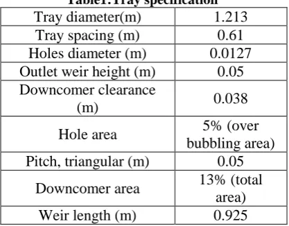
up to the upper tray and liquid flows down to the lower tray. Trays has a diameter of 1.213 m, a 13% downcomer area, a weir height of 0.05 m, a downcomer clearance of 0.038 m, and a 5% hole area with 0.0127-m-diam holes arranged in a 0.05-m triangular pitch. Table 1 presents tray specifications [13, 18].
Table1:Tray specification Tray diameter(m) 1.213
Tray spacing (m) 0.61
Holes diameter (m) 0.0127 Outlet weir height (m) 0.05 Downcomer clearance
(m) 0.038
Hole area 5% (over
bubbling area) Pitch, triangular (m) 0.05
Downcomer area 13% (total area)
Weir length (m) 0.925
In Figure 1, the y axis is the flow direction, z is perpendicular to the flow direction in a horizontal plane or transverse direction and x is the vertical axis.
Figure 1: The simulated sieve tray geometry
4. Grid size sensitivity
The available ANSYS Workbench [19] software automatically meshed the model geometry. It states that “Mesh density is
based on the de-featuring tolerance and maximum element size parameters. These parameters apply to the whole structure, although parts or bodies of the structure can be suppressed to prevent unnecessary meshes being created.
If suppressed, they will be excluded from the analysis and subsequent result will display. The default mesh settings were also mostly qualitative, which mean even lesser control of the mesh by the user.” Hybrid mesh has been employed for the gridding the geometry. Grids have tetrahedral shape, wedge, and are pyramid types. For testing the grid independency of the solutions, 3D meshes, which contained 112458, 202352, 269105, 350789 and 480256 cells, were used, respectively.
As it is shown in Figure 2, with increasing number of grids, the CFD predication results for clear liquid height became insignificantly better. After the specified number of elements, the results did not have obvious change. Therefore, the 269105 cells were used as a grid independent case for the computation.
Moreover, these selected cells were confirmed by the comparison between simulation result and experimental data.
Figure2: Test of number of cells on computational results for grid independency for constant
F-factor (Fs=1.015m/s2 QL= 0.0178).
5. Boundary conditions
wall, and symmetry planes [19]. The overall flow patterns on the distillation tray are highly sensitive to the inlet boundary conditions. The nature of mathematical modeling is such that the equations governing the phenomena must be solved over a domain of interest by isolating the domain from the surrounding through the proper choice of boundary conditions [20].
5.1. Liquid inlet
Uniform liquid inlet velocity profiles were applied as:
𝑈𝐿,𝑖𝑛 = 𝑄𝐿
𝑑𝑐 × 𝑊 , uL,y.in = 0 , 𝑢𝐿,𝑧,𝑖𝑛 = 0
(15)
Where W is the weir length and 𝑑𝑐 is the downspout clearance height. The liquid volume fraction at the liquid inlet was taken to be unit, since only liquid should enter the tray deck through the downspout clearance [4].
5.2. Gas inlet:
The gas velocity through each hole was calculated based on the assumption that mass flow rate through each holes are equal:
𝑢𝐺,𝑖𝑛 =𝑉𝐴𝑠𝐴𝐵
𝐻 (16)
Where, AH is the total holes area and AB
is the tray bubbling area. 𝑉𝑠 is the gas-phase
superficial velocity based on bubbling area. The gas inlet to the chamber area was calculated by Eq. 17.
VS=Fs/ 𝜌𝐺 (17)
The F-factor, Fs, is equivalent of the
square root of the kinetic energy of the vapor. Here, the velocity in Eq. 17 is based on the bubbling area AB. One should be
aware that Vs has been reported based on
the net area AN [1].
5.3. Outlet boundaries:
The vapor and liquid outlet boundaries are specified as mass flow boundaries with fractional mass flux specifications. The gas and liquid outlet specification were in agreement with the specification of inlet where only one fluid was assumed to enter [10, 21].
5.4. Wall boundary condition:
Wall boundary condition is used to bound fluid and solid regions. A no-slip wall boundary condition was specified for liquid phase while a free slip wall boundary condition was used for the gas phase.
6. Result and discussion
Simulation runs ended up by reaching steady state numerically. States of steady state were recognized by considering variation of clear liquid height with time. Figure 3 shows that at least about 21 seconds is required for reaching a quasi-steady state but most runs continued up to 30s.
Figure3: Clear liquid height variation as a function of time for constant F-factor (Fs=1.015m/s
2
QL= 0.0178). Number of cells are
269105.
Furthermore, the process of distillation sieve tray was studied in transient state. The high resolution and upwind advection schemes were used for solving equations. Time increment used in the simulation was 5.0×10⁻³s. The used boundary condition in the present work prevented the weeping phenomena. Physical properties of air and water at constant experimental condition of 25 oC were also employed [13].
6.1 Hydrodynamics
holdup in the system. The clear liquid height of sieve tray is related to the gas velocity, liquid load and weir height, its knowledge is required for the prediction of hydraulics parameters such as, average residence time distribution of liquid, pressure drop and efficiency. At steady state condition, clear liquid height remains practically constant for the long period of time. The froth region is usually defined as the region in which the liquid volume fraction is greater than 10%. Thus, the average froth height has been calculated as the area average over the tray deck ((y, z) plane) of the vertical at distance (x) from the tray floor at which the liquid volume fraction starts to fall below 10%. On industrial size sieve trays, the froth height is typically an order of magnitude smaller than the tray diameter [22]. Moreover, available experimental data of Solari and Bell [13, 18] has been used while liquid velocity profile, clear liquid height, froth height band and froth height were calculated by the use of CFD at varying rate of gas phase (FS=
0.464, 0.801, 1.015, 1.464 m/s (kg/m3)1/2) and liquid loads, QL, of 0.00694 m3 /s and
0.0178m3/s.
Simulation results were compared not only with the experimental data of Solari and Bell [13] but also with the data obtained by using correlations of Bennett et al., Eq. 13, [16] for average gas hold up. Furthermore, the model results were compared with the CFD simulation results model of Gesit et al. [4].
The noticeable point was that the CFD predicted results of the current work, shown in Figures 4 to 10, were closer to the experimental data of Solari and Bell and Bennett et al. correlation than those obtained by Gesit et al. [4] whom assumed symmetry in their models. That is because, even though, there appears symmetry in tray geometry the flow is in reality does not show a symmetrical behavior.
It is recommended in CFD modeling, if computational resources permit, one should use an actual geometry of the equipment.
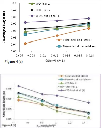
Figure 4 shows variation of clear liquid height with either liquid load or Fs. In Figure 4(a).
In Figure 4 (b), with the increase in Fs at
constant flow rate of liquid, (QL=0.0178m3/s), the clear liquid height
predictions are comparable. Notice should be made that hydrodynamic behavior of trays 1 and 2 are not similar. Thus, the efficiency of each tray is unique which depends on the tray hydrodynamics.
Figure4: (a) clear liquid height variation as a function of QL for constant F-factor (Fs=0.462
m/s(kg/m3)0.5). Comparison with experimental and CFD (b) Clear liquid height variation as a
function of Fs for constant liquid rate
(QL=0.0178m3/s) comparison with experimental
and CFD.
Fs was0.462 m/s (kg/m3)0.5. It is illustrated
that even at these low Fs the spray regime prevails because at low liquid load, the difference of all model predictions with the experimental results is high.
Figure 5 shows froth height variation as a function of Fs for constant QL=0.0178 m3/s.
by the Gesit, et al. [4] and Rahimi et al. [10] in their CFD models that had one tray in their geometry.
Figure5: Variation of froth height as a function of Fs for constant QL=0.0178 m3/s
Figure 6 represents the average liquid volume fraction in froth with the variation of Fs for constant QL=0.0178 m3/s.
Figure6: Variation of average liquid volume fraction in froth as a function of Fs for constant
QL=0.0178 m3/s.
In this figure, the different prediction of Benett et al. correlation is clear. The Bennet et al. correlation for clear liquid height is [16]:
0.67
(1.0 )[ ( ) ]
(1.0 )
average l
cl G w average
w G
Q
h r h C
L r
(18)
0.5 0.438exp( 137.8 w)
C h (19)
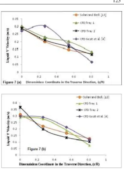
Figure7: Liquid velocity vector profile, QL =0.00694 m3 /s, Fs=1.015: (a) upstream profile;
(b) downstream profile.
Figure8: Liquid velocity vector profile, QL
=0.00694 m3 /s, Fs=1.462 m/s (kg/m3)0.5: (a) upstreamprofile; (b) downstream profile.
6.2 Velocity Profiles
The velocity of liquid, V, in the transverse direction to the liquid flow is presented in Figures 7 to 10.
The time average of liquid measurements velocity was made along the lateral (z) direction at two locations on the tray: 0.3235 m from the inlet downspout (referred to as the `Upstream’ location in subsequent discussion) and 0.21m from the outlet downspout (referred to as the `Downstream’location in subsequent discussion) [13].
Figure9: Liquid velocity profile, QL =0.0178 m3s-1,
Fs=0.462 m/s (kg/m3)0.5: (a) upstream profile; (b) downstream profile.
The velocity that was predicted by the present model and was compared with the experimental data shows reasonable agreement in spite of having some deviations. The discrepancy may be due to the following reasons. Solari and Bell [13] made linear liquid velocity measurements along two lines perpendicular to the liquid flow direction on a plane 0.038 m above the tray floor. As Solari and Bell [13] remarked, the gas rate plays an important role in determining the liquid-velocity distribution. It has been observed that at very low liquid rates, the liquid inlet velocity profile has a strong influence on the liquid flow profile within the tray [1].
Figure10: Liquid velocity profile, QL =0.0178 m3 /s, Fs=0.801 m/s (kg/m3)0.5: (a) upstream profile;
(b) downstream profile.
Figure11: Liquid velocity vectors on the tray decks. a) Tray 1, b) Tray 2. FS= 1.015 m/s
Figure12: Liquid volume fraction contour on a vertical section plan (y, x) 0.05 m from the tray center for FS= 0.462 m/s (kg/m3)0.5, QL=0.00694
m3/s
Figure11 (a) and 11.(b) illustrate the liquid velocity vectors on horizontal plane at 4 cm above the deck of trays 1 and 2. Those figures confirm that liquid flow on the trays is not only un-symmetrical but also is different at any time for each tray. Near the outlet downspout, there is an increase of flow in the vertical direction as the effect of the weir becomes significant. This observation suggested simulating whole columns, if computer hardware is not the controlling factor.
To visualize the flow of liquid a contour plot of liquid volume fraction is provided in Figure 12. Liquid volume fraction contour is for a vertical section in plan (y, x) that is 0.05 m from the central plan. Fs and QL
were 0.462 m/s (kg/m3)0.5 and 0.00694 m3/s, respectively.
7. Conclusion
A computational fluid dynamics (CFD) model was developed for describing the hydrodynamics of a column having two sieve trays. The tray geometries were based on the FRI commercial-scale sieve tray based on Solari and Bell’s sieve tray [13]. The assumption of symmetry for the tray simulation is not reliable and assumption of similar tray hydrodynamic for multi- tray columns is not valid. Additionally, it was concluded that whilst a column with more than one tray required more computational efforts, a more accurate estimation of tray
hydrodynamic parameters could be obtained only if a complete tower was simulated.
Nomenclature
AB [m2] tray bubbling area
AH [m2] total area of holes
CD [-] drag coefficient
dG [m] mean bubble
diameter
Fs [m/s
(kg/m3)0.5]
F-factor
g [m.s-2] gravity acceleration hcl [m] clear liquid height
hf [m] froth height
hw [m] weir height
Lw [m] weir length
MGL [kg.m-2.s-2] interphase
momentum transfer PG [N.m-2] gas- phase pressure
PL [ N.m-2] liquid- phase
pressure QL [m3.s-1] liquid volumetric
flow rate
rG [-] gas- phase volume
fraction
𝑟𝐺𝑎𝑣𝑒𝑟𝑎𝑔𝑒 [-] Average gas
hold-up fraction in froth
rL [-] liquid- phase
volume fraction
t [s] time
U [m/s] x-component of
velocity
V [m/s] y-component of
velocity
W [m/s] z-component of
velocity VG [m/s] gas- phase velocity
vector
VL [m/s] liquid- phase
velocity vector
Vs [m/s] gas- phase
superficial velocity based on bubbling
area Vslip [m/s] slip velocity
geometry is automatically taken into account by the CFD code. We conclude that CFD simulations prior to constructing the trays are beneficial. Experimental computational fluid dynamics of trays are waiting. As almost all published data are of Solari and Bell for one tray column.
Greek Symbols
μeff ,G [kg.m-1.s-1] Effective viscosity
of gas
μeff ,L [kg.m-1.s-1] Effective viscosity
of liquid ρG [kg.m-3] gas density
ρL [kg.m-3] liquid density
References
1. Kister, H. Z.(1992). Distillation Design, McGraw-Hill Inc.
2. Lockett, M. J.(1986). Distillation Tray Fundamentals, Cambridge University, Cambridge.
3. Stichlmair, J.G. and Fair, J.R. (1998). Distillation Principles and Practice, Wiley-VCH, New York.
4. Gesite G. K., Nandakumar, K., Chuang, K. T. (2003). "CFD Modeling of Flow Patterns and Hydraulics of Commercial-Scale Sieve Trays." AIChE. J., Vol. 49, pp. 910-924.
5. Li, X.G., Liu, D.X., Xu, S.M., Li, H. (2009). "CFD Simulation of Hydrodynamics of Valve Tray." Chem. Eng. Proc.: Process Intensification Vol. 48, pp. 145–151.
6. Krishna, R., Van Baten, J. M., Ellenberger, J., Higler, A.P., Taylor, R. (1999). "CFD Simulations of Sieve Tray Hydrodynamics." Chem. Eng. Res. Des., Trans. Inst. Chem. Eng., Vol.77, pp. 639–646.
7. Van Baten, J.M., Krishna, R. (2000). "Modeling Sieve Tray Hydraulics using Computational Fluid Dynamics." Chem. Eng. J., Vol.77, pp. 143–151.
8. Wang, X.L., Liu, C.J., Yuan, X.G., Yu, K.T. (2004). "Computational fluid dynamic simulation of three-dimensional liquid flow and mass transfer on distillation column trays." Ind. Eng. Chem. Res., Vol. 43, pp. 2556–2567.
9. Fischer, C. H., and Quarini, G. L. (1998). "Three Dimensional Heterogeneous Modeling of Distillation Tray Hydraulics." Miami Beach, FL: AIChE annual meeting, November 15–20.
10. Rahimi, R., Rahimi, M.R., Shahraki, F., Zivdar, M. (2006). "Efficiencies of sieve tray distillation columns by CFD simulation." Chem. Eng. Tech., Vol. 29, pp.326-350.
11. Noriler, D., Meier, H.F., Barros, A.C., Wolf, M. R. (2008). "Thermal fluid dynamics analysis of gas– liquid flow on a distillation sieve tray." Chem. Eng. J., Vol. 136, pp.133–143.
12. Malvin, A., Chan, A., Lau, P.L.,(2014). "CFD Study of Distillation Sieve Tray Flow Regimes using the Droplet Size Distribution Technique." J. Taiwan Inst. Chem. Eng., Vol. 45, pp. 1354-1368.
13. Solari, R. B., Bell, R. L. (1986). "Fluid Flow Patterns and Velocity Distribution on Commerical Scale Sieve Trays.", AIChE J., Vol. 32, pp. 640.
14. Liu, C. J., Yuan, X. G., Yu, K. T., Zhu, X. J. (2000). "A Fluid Dynamic Model for Flow Pattern on a Distillation Tray." Chem Eng. Sci. Vol. 55, pp. 2287-2294.
15. Krishna, R., Urseanu, M. I., Van Baten, J. M. and Ellenberger, J. (1999). "Rise Velocity of a Swarm of Large Gas Bubbles in Liquids." Chem. Eng. Sci., Vol. 54, pp.171-183.
16. Bennet, D. l., Agrawal and Cook, O. J. (1983)." New Pressure Drop Correlation for Sieve Tray Distillation Column." AIChE. J., Vol. 29, pp. 434-442.
18. Solari, R.B., Saez, E., D’apollo, I., Bellet, A. (1982). "Velocity Distribution and Liquid Flow Patterns on Industrial Sieve Trays." Chem. Eng. Commun. Vol. 13, pp. 369–384.
19. ANSYS CFX 11 User ҆ Guide, (2009). ANSYS, Ltd., Copyright.
20. Mehta, B., Chuang, K. T. and Nandakumar, K. (1998). "Model For Liquid Phase Flow On Sieve Trays."
Chem. Eng. Res. Des. Vol. 76, pp. 843-848.
21. Rahimi, R., Mazarei, M. and Bahramifar, E. (2008). "The effect of tray geometry on the sieve tray efficiency." Chem. Eng. Sci., Vol. 76, pp. 90-98 .