https://doi.org/10.5194/gmd-12-1267-2019 © Author(s) 2019. This work is distributed under the Creative Commons Attribution 4.0 License.
Terrainbento 1.0: a Python package for multi-model analysis in
long-term drainage basin evolution
Katherine R. Barnhart1,2, Rachel C. Glade2,3, Charles M. Shobe1,2, and Gregory E. Tucker1,2
1Cooperative Institute for Research in Environmental Sciences, University of Colorado at Boulder, Boulder, CO, USA 2Department of Geological Sciences, University of Colorado at Boulder, Boulder, CO, USA
3Institute for Arctic and Alpine Research, University of Colorado at Boulder, Boulder, CO, USA Correspondence:Katherine R. Barnhart ([email protected])
Received: 16 August 2018 – Discussion started: 12 October 2018
Revised: 14 February 2019 – Accepted: 15 February 2019 – Published: 3 April 2019
Abstract.Models of landscape evolution provide insight into the geomorphic history of specific field areas, create testable predictions of landform development, demonstrate the con-sequences of current geomorphic process theory, and spark imagination through hypothetical scenarios. While the last 4 decades have brought the proliferation of many alternative formulations for the redistribution of mass by Earth surface processes, relatively few studies have systematically com-pared and tested these alternative equations. We present a new Python package, terrainbento 1.0, that enables multi-model comparison, sensitivity analysis, and calibration of Earth surface process models. Terrainbento provides a set of 28 model programs that implement alternative transport laws related to four process elements: hillslope processes, surface-water hydrology, erosion by flowing water, and mate-rial properties. The 28 model programs are a systematic sub-set of the 2048 possible numerical models associated with 11 binary choices. Each binary choice is related to one of these four elements – for example, the use of linear or nonlinear hillslope diffusion. Terrainbento is an extensible framework: base classes that treat the elements common to all numeri-cal models (such as input/output and boundary conditions) make it possible to create a new numerical model without reinventing these common methods. Terrainbento is built on top of the Landlab framework such that new Landlab compo-nents directly support the creation of new terrainbento model programs. Terrainbento is fully documented, has 100 % unit test coverage including numerical comparison with analyti-cal solutions for process models, and continuous integration testing. We support future users and developers with intro-ductory Jupyter notebooks and a template for creating new
terrainbento model programs. In this paper, we describe the package structure, process theory, and software implementa-tion of terrainbento. Finally, we illustrate the utility of ter-rainbento with a benchmark example highlighting the differ-ences in steady-state topography between five different nu-merical models.
1 Introduction
models perform poorly, and to assess which transport laws are most appropriate for various environmental conditions, timescales, and spatial scales.
Relatively few studies have systematically compared and tested alternative transport laws, and those that do usually address only a single, quasi-one-dimensional landform el-ement, such as the shape of an idealized hillslope (Doane et al., 2018), the longitudinal profile of a particular stream channel (Tomkin et al., 2003; van der Beek and Bishhop, 2003; Loget et al., 2006; Valla et al., 2010; Attal et al., 2011; Hobley et al., 2011; Gran et al., 2013), or a fault scarp (Andrews and Hanks, 1985; Andrews and Bucknam, 1987; Hanks, 2013; Pelletier et al., 2006). Two-dimensional nu-merical models have focused on testing alternative formu-lations of soil production and transport (Herman and Braun, 2006; Roering, 2008; Petit et al., 2009; Pelletier et al., 2011), and studies that test two-dimensional numerical models that couple hillslope and channel processes are much more lim-ited (Hancock and Willgoose, 2001; Willgoose et al., 2003; Hancock et al., 2010; Gray et al., 2018). Models that com-bine hillslope and channel processes – often referred to as landscape evolution models – can simulate the formation of three-dimensional landforms that arise from the interaction of multiple processes, and in principle comparative testing ought to be straightforward (Hancock et al., 2010). Yet the algorithms behind these numerical models commonly differ from one another in multiple ways, which makes one-to-one comparison difficult. For example, if two numerical model codes differ simultaneously in their treatments of hydrology, sediment transport, and material properties, diagnosing any differences in their performance requires disentangling each of these effects. Often research questions focus on a combi-nation of geological process and boundary conditions; clas-sic examples include morphologic dating of fault scarps and glacial moraines. In this way, boundary conditions become a core numerical model component. To help address this chal-lenge, it would be useful to have a software framework in which an investigator could alter one “process ingredient” or boundary condition at a time and thereby conduct meaningful parameter studies, sensitivity analyses, calibrations, multi-model analyses, and comparisons with data.
Terrainbento is a Python-language software product de-signed to help meet this need. Terrainbento version 1.0 pro-vides three resources for exploring alternative process for-mulations for landscape evolution. First, terrainbento 1.0 in-cludes a collection of 28 distinct model programs for the long-term (order 104–106years) evolution of drainage basin topography; most of these programs vary from a simple “base” numerical model in just one or two particular process descriptions. We consider a systematic subset of the 2048 possible numerical models derived from 11 binary options (Sect. 3.9 describes the basis for the subset).
Second, terrainbento takes advantage of Python class in-heritance such that all common features of terrainbento model programs (such as input/output, and the handling of
boundary conditions) are provided in a generic “Erosion-Model” base class from which specific programs are derived. This ErosionModel class enables modelers to craft and ap-ply their own implementations without needing to reinvent the overarching software framework or the necessary util-ity functions. Terrainbento 1.0 builds on the Landlab toolkit (Hobley et al., 2017), using Landlab components to represent individual hillslope, hydrologic, and channel process com-ponents and taking advantage of Landlab to handle common tasks such as input and output management.
Finally, boundary conditions can have a profound impact on model behavior. Terrainbento has a set of extensible fea-tures called “boundary handlers” that can be used to imple-ment many common and complex boundary conditions.
Earth’s landscapes are incredibly diverse, and the scientific questions that they pose are equally extensive. No one model program, or even a general framework like terrainbento, can hope to encompass all of this diversity. Terrainbento 1.0 was originally created to address landscape evolution in a humid– temperate, soil-mantled, postglacial environment with mod-erate relief (order 102m, on a horizontal scale of order 104m) and relatively rapid erosion rates (10−4to 10−2m yr−1) over a timescale of order 104years. The choices of algorithms and process laws among the constituent numerical models reflect this motivation. Nonetheless, through the model template, terrainbento provides a sufficiently generic platform that it can be readily adapted to address a range of other scales and environments. This paper presents and describes terrainbento version 1.0, including its basic structure, mathematical un-derpinnings, software implementation, and the 28 constituent model programs.
2 General structure of a terrainbento model program A terrainbento model program begins with a gridded representation of topography. Landlab’s RasterModelGrid, HexModelGrid, RadialModelGrid, and irregular Delaunay– Voronoi grids are all supported in terrainbento version 1.0. The elevation, and regolith thickness if present, at each grid node evolves according to a specified set of erosion and/or sediment transport laws, which vary between model pro-grams. Terrainbento is agnostic to time and space units but expects that a user will ensure consistency between the grid units, time step units, and model input parameters.
2.1 A note on terminology
The word “model” can have multiple meanings in scientific computing and indeed in science generally. Here we will use the term mathematical modelto mean a set of govern-ing equations, which in this case describe landscape evolu-tion under a given set of assumed process dynamics, material properties, and boundary conditions. Under this definition, two mathematical models may have governing equations that are structurally quite similar, but which are nonetheless con-sidered to be distinct models either because certain constants take on different values or because a term is included in one version but not the other. For example, as described below, water erosion is commonly treated as proportional to either hydraulic power or hydraulic stress. We consider these to be distinct mathematical models, despite the fact that the differ-ence lies only in the choice of two exponent values in the governing equation.
Each mathematical model contains terms that represent individual processes (or closely related collections of pro-cesses), such as erosion by surface-water flow. The mathe-matical representation for an individual process will be re-ferred to as a process law or rate law. By this definition, a mathematical model in terrainbento consists of a set of process laws embedded within an overall mass-conservation equation.
The termnumerical modelis used here to refer to a numer-ical algorithm that solves a particular mathematnumer-ical model by marching forward in time from a given initial condition un-der given boundary conditions. The termmodel programwill refer to a set of source code files that performs the calcula-tions needed to implement a numerical model. In some cases in terrainbento 1.0, a single model program can be config-ured to implement many numerical models, depending on its input parameters. One can consider alternative models that require only a different set of model program parameter val-ues alternativeparametric models, whilst models that require a different program are differentstructural models. The com-bination of a model program plus the inputs that control this type of choice will be referred to as amodel configuration. 2.2 Basic ingredients and governing equation
Topography in a terrainbento mathematical model is rep-resented as a two-dimensional field of elevation values,
η(x, y, t ). The general governing equation describes the rate of change ofηas the sum of two terms: one representing ero-sion (or deposition) of mass by water-driven processes and one representing gravitational (“hillslope”) processes:
∂η
∂t = −EW−EH, (1)
whereEWis the rate of erosion (or deposition, if negative) by water-driven processes such as channelized flow, and EH is the rate for gravitationally driven processes such as soil creep
and shallow landsliding (the subscript H stands for “hills-lope,” recognizing that gravitational processes will tend to be most important on hillslopes). Water erosion is assumed to depend on local slope gradient, S, water discharge, Q
(which in many terrainbento model programs will be treated using drainage area as a surrogate, as discussed below and in Sect. 3.6), and material properties. Erosion or accumulation by gravitational processes is assumed to be a function of gra-dient, material properties, and (in some model programs) soil thickness.
While many terrainbento model programs only treat the evolution of the topographic surfaceη, two types of model program treat a more complex set of layers. The first type adds an explicit mobile-regolith layer on top of bedrock. The second type treats two different bedrock lithologies in a user-determined spatial configuration.
2.2.1 Soil-tracking model programs
Several of terrainbento’s model programs explicitly track a layer of regolith, defined here as unconsolidated and po-tentially mobile sediment, such as soil or alluvium (see Sect. 3.7.1). Here, for simplicity we will refer to this mate-rial as soil, keeping in mind that our operational definition is more general than the one commonly used by soil scientists (Soil Survey Staff, 1999). The land surface height is the sum of bedrock elevation,ηb, and soil thickness,H:
η=ηb+H . (2)
Here too the term “bedrock” is used in its broadest possi-ble sense and may include, for example, cohesive sedimen-tary material such as glacial till or saprolite. The time rate of change of soil thickness is the difference between the rate of soil production and erosion,
∂H
∂t =P−EWHS, (3)
whereP is the rate of soil production from bedrock, and
EWHSdenotes the total rate of soil erosion (or accumulation, if negative) resulting from water-driven and gravity-driven transport processes. Similarly, the rate of change of bedrock surface height is the sum of the soil production rate (scaled by any density contrast between rock and soil) and the rate of bedrock incision by running water,EWR:
∂ηb
∂t = − ρs
ρr
P −EWR. (4)
2.2.2 Multi-lithology model programs
Nine terrainbento model programs allow for spatial juxtapo-sition of two different lithologies,L1 andL2. Layer L1 is assumed to overlieL2, but it may be absent (thickness zero) at any particular location. LetηL2(x, y, t )denote the
ofL1. Then the land surface elevation (in the absence of an explicit soil layer) is given by
η=ηL2+TL1. (5)
In model programs that honor both a soil layer and two dif-ferent lithologies, the surface elevation is
η=ηL2+TL1+H , (6)
in which case the height of the bedrock surface is
ηb=ηL2+TL1. (7)
Where the top layer exists, it lowers as a result of water ero-sion and (if soil is tracked) rock-to-soil converero-sion. This can be expressed mathematically as
∂TL1
∂t = −δL(EW+P ) , (8)
where δL is a spatially varying function equal to 1 where
L1>0 and 0 elsewhere (hereP is considered to be zero in non-soil-tracking model programs). The rate of change of el-evation of the top ofL2is given by
∂ηL2
∂t = −(1−δL) (EW+P ) , (9)
which means that the lower layerL2is vulnerable to erosion and weathering wherever the top layer is missing (for exam-ple, having been eroded through). Note that the BasicHySa model program allows for the simultaneous water erosion of soil and rock, as discussed below.
3 Process formulations
Each of the 28 model programs in the terrainbento 1.0 col-lection has four elements, reflecting the treatment of hills-lope processes, surface-water hydrology, erosion by running water, and material properties. The possible formulations for each of these elements are constructed around a set of binary choices. Each choice represents a decision about how a par-ticular element might be formulated. For example, the down-hill soil transport rate could be represented as either a linear or nonlinear function of local topographic gradient, while the lithology could either be treated as uniform or divided into two distinct types as discussed in Sect. 2.2.2. The binary-choice design makes it possible to test the behavior of one alternative process element at a time. The binary options that form the basis for the terrainbento 1.0 constituent model pro-grams are listed in Table 1. In Table 1, option B in each row usually represents a more sophisticated choice than option A: one that may bring more realism, but generally involves more parameters.
Each of terrainbento’s model programs uses Landlab com-ponents to implement the numerical algorithms behind chan-nel erosion, hillslope processes, and water-flow routing.
The components used are briefly identified by name in the following descriptions. The software architecture that sup-ports this component-based approach is then discussed fur-ther in Sect. 5. Furfur-ther information about Landlab and its component-modeling capability is provided by Hobley et al. (2017).
3.1 Model domain options
Terrainbento supports all types of Landlab model grids. Many options for the creation of synthetic topography and instantiation from a DEM are available. These options are described in the user manual.
3.2 Drainage area, flow direction, and flow accumulation
All terrainbento model programs calculate drainage area and surface-water discharge using the Landlab FlowDirectors and FlowAccumulator. Flow direction algorithms presently supported in Landlab include SteepestDescent/D4, D8, D∞, and Multiple Flow Direction (O’Callaghan and Mark, 1984; Freeman, 1991; Tarboton, 1997). Water routing across closed depressions is optionally handled using a lake-fill algorithm implemented by the Landlab DepressionFinderAndRouter component (the current version of which uses an implemen-tation based on Tucker et al., 2001). Once flow directions and surface-water runoff are calculated, the contributing drainage area or surface-water discharge at a given grid celliis calcu-lated by adding up the area of all cells whose flow eventually passes throughi, plus the area or discharge ofiitself using the Landlab FlowAccumulator component.
3.3 Basic model program
The simplest of the component model programs in terrain-bento is known as the Basic model program. It implements a discretized numerical solution to the following governing equation for land surface elevationη(x, y, t ):
∂η
∂t = −KQ
mSn+D∇2η , (10)
Table 1.Model program binary options.
Category Option A Option B
Hillslope processes linear transport law nonlinear transport law
Surface-water hydrology deterministic stochastic
uniform runoff variable source area runoff
Erosion by flowing water ωc=0 ωc>0 stream power shear stress
constantωc ωcincreases with incision depth detachment-limited sediment-tracking
uniform sediment∗ fine vs. coarse∗
Material properties no separate soil layer tracks soil layerH (x, y, t ) homogeneous lithology two lithologies
Paleoclimate constant climate time-varyingK
∗Only applies to sediment-tracking model programs (see text).
Table 2.Summary of 28 individual model programs in the terrainbento 1.0 collection.
Model Element varied
configuration
No. 1 No. 2 No. 3
Basic – – –
BasicTh variableωc – –
BasicDd ωct∝incision depth – –
BasicHy sediment-tracking channel erosion rule – –
BasicCh nonlinear (cubic) hillslope soil transport – –
BasicSt stochastic runoff generation – –
BasicVs variable source area runoff generation – –
BasicSa tracks soil and alluvium – –
BasicRt tracks two lithologies – –
BasicCc Kvaries over time – –
BasicStTh variableωc stochastic runoff generation – BasicThVs variableωc variable source area runoff generation –
BasicRtTh variableωc tracks two lithologies –
BasicDdHy ωct∝incision depth sediment-tracking channel erosion rule – BasicDdSt ωct∝incision depth stochastic runoff generation – BasicDdVs ωct∝incision depth variable source area runoff generation – BasicDdRt ωct∝incision depth tracks two lithologies – BasicHySt sediment-tracking channel erosion rule stochastic runoff generation – BasicHyVs sediment-tracking channel erosion rule variable source area runoff generation – BasicHySa sediment-tracking channel erosion rule tracks soil and alluvium – BasicHyRt sediment-tracking channel erosion rule tracks two lithologies – BasicChSa nonlinear (cubic) hillslope soil transport tracks soil and alluvium – BasicChRt nonlinear (cubic) hillslope soil transport tracks two lithologies – BasicStVs stochastic runoff generation variable source area runoff generation – BasicSaVs variable source area runoff generation tracks soil and alluvium – BasicRtVs variable source area runoff generation tracks two lithologies – BasicRtSa tracks soil and alluvium tracks two lithologies –
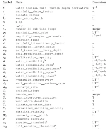
model run and slope–area diagrams like that shown in Fig. 2, can be found in the Jupyter notebook tutorials on GitHub (Barnhart et al., 2019b).
The second term on the right is the popular linear diffu-sion rule for hillslopes (Culling, 1963). The first term on the right represents channel incision and is based on the widely used stream-power formulation (Howard et al., 1994; Whip-ple and Tucker, 1999), in which the long-term average rate of channel downcutting is taken to be proportional to hy-draulic power per unit bed area. A key assumption behind the Basic model program is that the erosion rate is limited by the capacity to detach and remove material, rather than by along-stream variations in the capacity to transport sediment. A common simplification, discussed further in Sect. 3.6, is that drainage area,A, appears as a surrogate for effective wa-ter discharge. Often the choice m=1/2 is made, reflecting the assumption that discharge per unit channel width scales as the square root of drainage area (Wohl and David, 2008). Similarly, n is commonly taken to be unity based on the derivation from stream power. The examples presented below use the exponent valuesm=1/2 andn=1 unless otherwise noted.
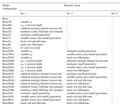
Rather than hard coding values for the water-erosion dis-charge exponentmand slope exponentn, terrainbento model programs permit varying these two exponents as parameters. Thus, within terrainbento 1.0 the same model program can be configured to represent either a stream-power or shear-stress representation of water erosion. Similarly, alternative forms of the fluvial erosion process law can be implemented by changing the value ofmornto reflect (for example) a differ-ent channel width–discharge scaling relation (Snyder et al., 2003b; Wohl and David, 2008) or different fluvial erosion mechanisms (Whipple et al., 2000a). For example, Fig. 1b shows an example of an alternative parametric model that uses the Basic model program with a value ofm=1/4.
Although Eq. (10) is rather simple, having just four param-eters (K,D,m, andn), it represents a formulation that has been widely used in geomorphic modeling (e.g., Miller and Slingerland, 2006; Miller et al., 2007; Perron et al., 2009; Pelletier, 2010; Duvall and Tucker, 2015). The equations are commonly solved numerically on a regular or irregular grid. Discharge and drainage area are normally evaluated using a downslope routing algorithm in which the water output from one grid cell is passed to one or more downhill neighbor-ing cells (see, for example, review in Tucker and Hancock, 2010). Despite its simplicity, this two-parameter numerical model has been shown to reproduce first-order properties of drainage basin topography, including dendritic drainage networks, concave-upward channel longitudinal profiles, and convex-upward hillslopes.
One arrives at the terrainbento Basic model program by choosing option A for each item in Table 1. In the fol-lowing subsections, we review the various options that ter-rainbento offers for alternative treatment of hillslope
pro-cesses, surface-water hydrology, channel incision, materials, and boundary conditions.
3.4 Hillslope processes
To simulate hillslope evolution processes in a soil-mantled landscape, we use components of varying complexity that treat soil transport as a diffusion-like process in which sedi-ment flux is governed by topographic gradient. Terrainbento offers two alternative soil flux rules with which to simulate the downslope transport of soil and its dependence on topo-graphic gradient: linear and nonlinear.
In addition, as discussed previously, terrainbento also al-lows for the option of explicitly tracking a dynamic soil layer. Our representation and treatment of soil evolution are simpler than in existing models focused on soil production and evolution (e.g., Cohen et al., 2010; Vanwalleghem et al., 2013). The dynamic soil option is provided to address the possibility that soil may become thin enough to limit flux, and this limitation may in turn influence the rate and style of landscape evolution. Inclusion of a dynamic soil layer re-quires an equation for soil production from the underlying lithology (P in Eq. 3) and, furthermore, that the flux law be modified to account for the local soil thickness such that soil flux goes smoothly to zero as thickness declines.
3.4.1 Continuity law for soil creep
The simplest forms of the so-called “geomorphic diffusion” equation (Dietrich et al., 2003) assume transport-limited con-ditions, in which the production rate of soil is always much greater than the transport rate; thus, the transport rate does not depend on soil availability or thickness. In this case, the hillslope term in the continuity Eq. (1) is
EH= 1
1−φ∇qh, (11)
whereqhis the hillslope soil volume flux per unit width,φis the porosity of the soil, and the∇operator represents differ-entiation in both horizontal directions (∇ =∂/∂x+∂/∂y). 3.4.2 Linear creep law
A variety of formulae exist for the soil flux,qh. The sim-plest and most common formula (Culling, 1963) treats the soil transport rate as a simple linear function of topographic gradient using a transport efficiency constant,D0:
qh= −D0∇η , (12)
where∇η is the slope gradient. Using this flux rule with Eq. (11), the hillslope term in the continuity equation be-comes
EH= −D∇2η , (13)
Figure 1.Three-dimensional view of simulated topography illustrating the use of five different terrainbento model programs:(a)Basic, (b)Basic withm=0.25,(c)BasicCh,(d)BasicVs, and(e)BasicRt. Each landscape was initialized with the same random noise field, has the same boundary conditions of the center core nodes uplifted relative to a fixed boundary, and was run to steady state (based on topographic change between 1000-year intervals exceeding 1 mm at no grid cell). Each domain is 1×1.6 km, has 10 m grid spacing, and is displayed with a vertical exaggeration of 5 to 30×.
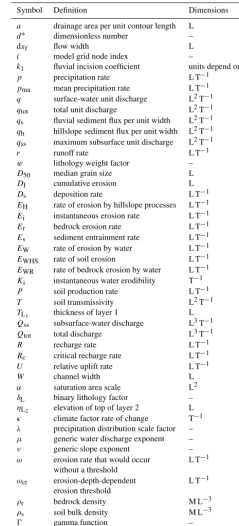
Figure 2. Slope–area relationship for the example simulation in Fig. 1a.
simplest form of the evolution equation for soil creep on hill-slopes results in convex-upward topography at steady state.
3.4.3 Nonlinear creep law
land-scape evolution model program, whereby other processes may produce gradients equal to or greater thanSc. Some au-thors have addressed this problem with a modified form that avoids divergence at gradientS=Sc(e.g., Carretier and Lu-cazeau, 2005).
Terrainbento uses a truncated Taylor series formulation for soil flux, which was derived by Ganti et al. (2012) for the Andrews–Bucknam law. The flux is given by
qh= −DS
"
1+
S Sc
2
+
S Sc
4
+. . .
S Sc
2(N−1)#
, (14) whereS= −∇ηis topographic gradient (positive downhill),
Dis the transport efficiency factor, andScis a critical gradi-ent. The user specifies the number of termsN to be used in the approximation. The nonlinear flux rule results in convex-up topography for shallow slopes and transitions to linear hillslopes for steeper slopes. An example terrainbento sim-ulation using the nonlinear creep law is shown in Fig. 1c. 3.4.4 Linear depth-dependent creep law
For model programs that explicitly track a soil layer
H (x, y, t ), one needs to modify the creep law to incorpo-rate a relationship between flux,qh, and local soil thickness. Terrainbento uses an approach proposed by Johnstone and Hilley (2015), in which the flux decays exponentially as soil thickness approaches zero:
qh= −D
1−exp
−H
H0
∇η , (15)
whereH0represents the soil thickness for whichqhshrinks to(1−1/e)of its maximum value for a given slope gradient. (Note that in the original formulation of Johnstone and Hil-ley (2015),Dis treated as the product ofH0and a transport coefficient with dimensions of length per time; here we lump them together asD.)
3.4.5 Nonlinear depth-dependent creep law
We can modify the nonlinear flux rule (Eq. 14) to accommo-date soil, again assuming an exponential velocity distribution in the subsurface (Johnstone and Hilley, 2015):
qh= −DS
1−exp
−H
H0
"
1+
S
Sc
2
+
S
Sc
4
+. . .
S
Sc
2(N−1)#
. (16)
This approach is somewhat similar to that used by Roering (2008) in a study that compared the predictions of a nonlin-ear, depth-dependent flux law with observed hillslope forms. 3.4.6 Soil production
Models that track a layer of soil must include an expression to specify the rate at which soil is produced from the
under-lying parent material. The most commonly applied formula, and the one used by terrainbento’s soil-tracking model pro-grams, treats the rate of soil production from the underlying lithology as an inverse-exponential function of soil thickness (Ahnert, 1976; Heimsath et al., 1997; Small et al., 1999):
P =P0exp(−H /Hs) , (17)
whereP0is the maximum production rate (with dimensions of length per time), andHsis a depth–decay constant on the order of decimeters.
3.5 Hydrology
Treatments of surface-water hydrology in landscape evolu-tion models are commonly quite straightforward, reflecting the need for both simplicity and computational efficiency. Erosion formulae normally require specification of water dis-charge or (less commonly) depth. The most common param-eterization is to use contributing drainage area,A, as a sur-rogate for surface-flow discharge,Q. This effectively states that Q=rA, where r, a runoff rate per unit area, is equal to 1. This is the default option in terrainbento’s model pro-grams. Operationally, this means that the water-erosion law includesAas the effective discharge (see Sect. 3.6 below) and that the erosion law parameters embed information about climatic factors such as precipitation frequency and intensity, as well as material properties such as soil infiltration capacity (e.g., Tucker, 2004).
3.5.1 Variable source area hydrology
topographic gradient,S. The maximum subsurface discharge per unit contour width is therefore given by
qss=KsatH S=T S , (18)
where T =KsatH is the soil transmissivity. Next, we con-sider a recharge rate,R, which represents the average rate of water input per unit area (dimensions of length per time). The total unit discharge is the product of recharge and drainage area per unit contour length,a:
qtot=aR . (19)
Using these two principles, the surface-water unit discharge,
q, at any location is
q=
0 if aR < T S
aR−T S otherwise. (20)
This threshold-based approach has been used, for exam-ple, in numerical models that explore how hillslope hy-drology influences landform evolution (Ijjasz-Vasquez et al., 1993; Tucker and Bras, 1998). One drawback, however, is that the use of mathematical thresholds in numerical models can complicate the calibration process by creating “numeri-cal daemons”: sharp discontinuities in a numeri“numeri-cal model’s response surface (i.e., the Np-dimensional surface that de-scribes a simulation output quantity as a function of itsNp
in-put parameters) (e.g., Kavetski and Kuczera, 2007; Hill et al., 2016). In this particular case, we can create a smoothed ver-sion of Eq. (20) without any loss of realism by positing that within any given patch of land there is actually a distribu-tion of effective recharge rates. The use of a smooth version in this formulation has two benefits – it is physically more realistic and is less prone to numerical discontinuities. The simplest strictly positive probability distribution is an expo-nential function
p(R)=(1/Rm)e−R/Rm, (21)
wherep(R)is the probability density function ofR, andRm is the mean recharge rate. The mean surface-water unit dis-charge can then be found by integrating as follows:
q= ∞
Z
Rc
q(R)p(R)dR=aRme−T S/Rma, (22)
whereRc=T S/a is the minimum recharge needed to pro-duce surface runoff.
It is useful to recast this in terms of an effective contribut-ing area,Aeff, defined as
Aeff=
q1x Rm
=Ae−T 1xS/RmA, (23)
where 1x represents flow width (in a gridded digital ele-vation model, it would be natural to use cell width). Note
that we have assumed that the contour width is approximated by the flow width. By this definition, the effective drainage area is always less than or equal to the actual drainage area, reflecting the fact that some of the water runs through the shallow subsurface rather than across the surface as over-land (or channelized) flow. Where slope gradient is small or drainage area is large, the effective area approaches the ac-tual area. If the surface is flat (S=0), the exponential factor equals unity andAeff=A, reflecting the fact that no water can be conveyed by shallow subsurface flow. At locations where the gradient declines in the downslope direction, wa-ter previously carried by subsurface flow effectively “exfil-trates” from subsurface flow within the soil layer and is car-ried as surface-water discharge. Conversely, whereSis large and/orAis small – as might be the case in steep headwa-ter areas – the effective drainage area becomes much smaller than the actual area, indicating that most of the incoming wa-ter is traveling beneath the surface rather than contributing to overland flow.
A final step is to note that one can collapse the various factors in Eq. (23) into a single parameter, α=T 1x/Rm, the saturation area scale (dimensions of length squared). A high value of α represents soils that have a large capacity to carry subsurface flow relative to the recharge rate; a low value reflects a more limited subsurface flow capacity.
Seven of terrainbento’s model programs implement vari-able source area hydrology by using Aeff, as defined in Eq. (23), in place of drainage area,A(Table 2). One of these (BasicSaVs) also explicitly tracks a soil layer, and the time-and space-varying thickness of this soil layer,H (x, y, t ), is used to calculateT =KsatH (x, y, t ). An eighth model pro-gram (BasicStVs) also uses a stochastic treatment of precip-itation; in this model program, the randomly generated pre-cipitation ratepis used forRmin Eq. (23).
An example simulation with a terrainbento model program (BasicVs) that includes a variable source area component is shown in Fig. 1d. The only difference in formulation be-tween this example and the Basic model program illustrated in Fig. 1a is that BasicVs calculates channel erosion using ef-fective drainage area,Aeff, as defined in Eq. (23), in place of total drainage area. The result is a drainage network bounded by steep, convex-upward ridges. These ridges are sufficiently steep that AeffA, so their erosion is dominated by soil creep. The bases of the hills represent locations where wa-ter emerges from the shallow subsurface to become surface flow that feeds the channel network.
3.5.2 Stochastic precipitation and runoff
ap-proach has the advantages of simplicity and computational efficiency, but also has limitations. For example, the appro-priate effective discharge may vary in space and time (Huang and Niemann, 2006). One solution is to use a stochastic treat-ment of precipitation and/or discharge, in which events are drawn from a specified probability distribution (Tucker and Bras, 2000; Snyder et al., 2003a; Tucker, 2004; Lague et al., 2005).
In order to facilitate comparison between numerical mod-els with deterministic and stochastic treatments of water dis-charge, terrainbento 1.0 includes a set of six model pro-grams that each implement two stochastic precipitation al-gorithms available in the PrecipitationDistribution Landlab component. The aim of these algorithms is not to reproduce individual storm events, but rather to capture a spectrum of runoff and streamflow events of varying frequency and mag-nitude. The first of these two methods is a stochastic-in-time approach based on Tucker and Bras (2000). The second op-tion uses deterministic time steps but stochastic precipitaop-tion intensity.
In the first option, a series of “storms” is generated based on a specified mean storm durationTr, mean inter-storm du-ration Tb, and mean storm depthhr. The mean storm and inter-storm durations are generated from exponential distri-butions, after Eagleson (1978). For each individual storm, the mean storm depth is generated from a gamma distribution. The gamma shape parameter used to draw a random storm depth is equal to that specific storm’s duration divided by the mean storm duration. The scale parameter is equal to the mean storm depth. The depth and duration of an individual storm are then used to calculate the rainfall intensity (Ivanov et al., 2007).
In the second option, in which the time step duration is fixed, the frequency of occurrence of rainfall is described us-ing an intermittency factor,F, which is defined as the frac-tion of time rain occurs rain, and a mean event precipitafrac-tion rate,pd.
Thus, the mean precipitation rate (averaged over wet and dry periods),pma, is given as
pma=F pd. (24)
The probability distribution of precipitation rate,p, is sim-ulated using a stretched exponential survival function, Pr(P > p)=exp
h
−
p
λ
ci
, (25)
wherecis a shape parameter andλis a scale parameter. Use of the stretched exponential function is based on Rossi et al. (2016), who found that the function provides a good approx-imation for daily rainfall distributions in the continental US and Puerto Rico. While Rossi et al. (2016) found this dis-tribution to be appropriate for meandailyrainfall, note that terrainbento is agnostic to the time units chosen by a user. Wilson and Toumi (2005) argued that theoretical
considera-tions suggestc≈2/3, while Rossi et al. (2016) found a mean value ofc=0.74 for weather stations in the continental US.
The shape parameterλassociated with a mean daily pre-cipitation ratepdand shape factorcis given by
λ= pd
0(1+1
c)
, (26)
where0is the gamma distribution function.
To describe the frequency–magnitude spectrum proba-bilistically in terrainbento’s stochastic model programs, time is discretized into a series of steps of durationδt /nts, where
δtis the “global” time step used for all other process compo-nents. During each step, an “event” with precipitation rate
p is drawn at random from the cumulative distribution in Eq. (25). One of two approaches is then used to calculate the corresponding runoff rate,r. The first approach, which is the default used in five of the six stochastic model programs, as-sumes a mean soil infiltration capacityIm. The rate of runoff is calculated as
r=p−Im
1−e−p/Im. (27)
This formulation is a smoothed version of the simple thresh-old approachr=max(p−Im,0), which has been used in prior studies to represent infiltration-excess overland flow generation (e.g., Tucker and Bras, 2000). The smoothed ver-sion avoids the sharp discontinuity atp=Imand is arguably more realistic as it honors natural variability in soil infiltra-tion capacity. The runoff rate approaches zero whenpIm and approachespwhenpIm.
The second approach uses the variable source area runoff generation formulation described in Sect. 3.5.1 usingp in place of recharge Rm. This approach is used only in the model program BasicStVs (Table 2).
3.6 Water erosion
and in some of these the threshold increases with progressive incision depth. Each variation is presented and discussed in the sections below. Here, we start with a description of the simplest formulation, which serves as the default choice.
The area–slope (a.k.a., stream-power) family of erosion laws derives from the assumption that the erosion rate,EW, depends primarily on the hydraulic gradient,S, the water dis-charge,Q, and the channel widthW:
EW=k1(Q/W )µSν−ωc, (28)
where k1 is a coefficient that depends on material proper-ties, channel geometry, and other factors, andωcis a old below which no erosion occurs (in practice, the thresh-old is often assumed negligible, or its effects are taken to be subsumed in the exponents). The exponentsµandν reflect the nature of the erosional processes; for example, Whipple et al. (2000a) argued that different values may be appropriate for abrasion-dominated and for plucking-dominated systems. The discharge exponent µ also embeds information about channel geometry. Often, drainage area Ais used as a sur-rogate for discharge. One limitation of Eq. (28) is that it does not allow for sediment deposition; for this reason, it is some-times referred to as a detachment-limited law (a term first coined by Howard, 1994), reflecting the assumption that the rate of downcutting is limited by the rate at which material can be detached and removed.
Despite the simplicity of Eq. (28), its various permutations have shown reasonable success when tested against field ob-servations (Stock and Montgomery, 1999; Whipple et al., 2000b; Kirby and Whipple, 2001; Snyder et al., 2000; Lavé and Avouac, 2001; Tomkin et al., 2003; van der Beek and Bishhop, 2003; Duvall et al., 2004; Loget et al., 2006; Whit-taker et al., 2007; Attal et al., 2008, 2011; Yanites et al., 2010; Hobley et al., 2011; Gran et al., 2013). Landscape evolution models that use the generic stream-power approach are able to reproduce basic properties of erosional landscapes, such as dendritic channel networks with concave-upward longitudi-nal profiles (e.g., Howard, 1994; Whipple and Tucker, 1999; Tucker and Whipple, 2002).
One of the most commonly used versions of Eq. (28) is obtained by making the following assumptions: (1) channel width can be represented as a power function of drainage area, and (2) the erosion threshold is negligible. Under these conditions, the erosion law becomes
EW=KQmSn, (29)
whereKis a coefficient that includes information about pre-cipitation and hydrology as well as material properties and channel geometry. The change fromνtonreflects the pos-sibility that slope-dependent information is included in K. This is the fluvial erosion law introduced earlier in the dis-cussion of the Basic model program. If one also assumes that
Q=rA, withrrepresenting runoff rate, then Eq. (29) can be
cast in the commonly used form
EW=K0AmSn, (30)
whereK0=Krm.
With respect to the exponents m andn, if one assumes that (1) the rate of downcutting depends on stream power per unit surface area, (2) effective discharge is proportional to drainage area, and (3) channel width is proportional to the square root of discharge, then the exponent values become
m=1/2 andn=1.
The simplicity of Eq. (29) – it has only one parameter if
mandnare assumed to be accurate representations of pro-cess – together with its ability to reproduce common features of drainage basins and networks have led to its widespread use in landscape evolution studies, especially with the ex-ponent valuesm=1/2 andn=1 (e.g., Duvall and Tucker, 2015). One might think of this particular configuration as the “model to beat”: to justify a more complex formulation, one would ideally need to demonstrate that such a formulation performs distinctly better.
Equation (29), which we will refer to as the simple stream-power law, forms the default choice for water erosion in ter-rainbento’s model programs. In the following subsections, we describe the variations and alternatives to simple unit stream power among the terrainbento 1.0 model programs. The complete governing equations for each of the terrain-bento 1.0 model programs are given in Appendix A. 3.6.1 Erosion threshold
Bed-load sediment transport is well known to exhibit threshold-like behavior, in which the transport rate is neg-ligible until a certain minimum hydraulic tractive stress is reached, at which point significant transport begins. Similar behavior applies to the erosion of highly cohesive sediment (e.g., Julien, 2010) and presumably also to bedrock (though the values of the operative thresholds for bedrock are not known). For this reason, models of landscape or longitudi-nal channel profile evolution often include a threshold term below which no erosion takes place.
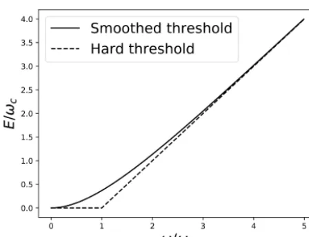
Several terrainbento model programs include a threshold in the water-erosion law. In order to promote mathemati-cally smooth behavior, acknowledge evidence for distribu-tions of transport thresholds (Kirchner et al., 1990; Wilcock and McArdell, 1997; McEwan and Heald, 2001), and avoid numerical daemons associated with threshold-type equations (e.g., Kavetski and Kuczera, 2007), the basic thresholded erosion law in terrainbento uses an exponential smoothing function following Shobe et al. (2017). Terrainbento’s thresh-olded erosion laws take the form
EW=ω−ωc(1−e−ω/ωc) . (31)
Figure 3.Illustration of the functional form of the smooth-threshold erosion law (Eq. 31) compared with the more traditional hard-threshold formulation.
and either drainage area or discharge. For example, for those model programs that add a threshold term to the area–slope erosion in Eq. (29),ωis defined as
ω=KQmSn. (32)
The factorωcis a threshold with dimensions of length per time. The functional form of the smooth-threshold erosion function (Eq. 31) is illustrated in Fig. 3. A constant threshold term is included in the water-erosion laws for five of terrain-bento’s constituent model programs (Table 2). Several others use a space- and time-varying threshold, as we describe next. 3.6.2 Incision depth-dependent erosion threshold In a study of river incision into glacial deposits following ice recession in the US upper midwest, Gran et al. (2013) found evidence for an erosion threshold that increased with pro-gressive incision depth. They attributed this to a downstream increase in median grain diameter resulting from enrichment of coarse gravel in bed material as the channel cuts through glacial deposits and the valley widens. In comparing alter-native long-profile-evolution numerical models with the ob-served profile, they found that the best match was achieved when the erosion threshold was allowed to increase linearly as a function of cumulative incision depth. Inspired by the findings of Gran et al. (2013), terrainbento 1.0 includes the option to allow the erosion thresholdωctto increase with ero-sion depth according to
ωct(x, y, t )=max(ωc+bDI(x, y, t ), ωc) , (33) whereDIis the cumulative incision depth at location(x, y) and time t,ωc is the threshold when no incision has taken place yet, and b (with dimensions of inverse time) sets the rate at which the threshold increases with progressive inci-sion depth. As before, an exponential term is used to smooth
the threshold such that the water-erosion rate approaches zero whenωωcand asymptotes toω−ωcwhenωωc (Fig. 3). The max function is included to prevent the thresh-old from decreasing in locations where hillslope processes produce net deposition (i.e., negative incision).
3.6.3 Shear-stress erosion law
Two important and commonly used measures of the ero-sional potential of streamflow are unit stream power and shear stress. The first represents the rate of energy dissipa-tion per unit surface area, while the second represents the hy-draulic traction force per unit area. Erosion rates in cohesive or rocky material tend to correlate strongly with both quanti-ties (e.g., Howard and Kerby, 1983; Whipple et al., 2000b), and both are widely used as the basis for long-term erosion laws. To support studies that compare and test these two ap-proaches, terrainbento 1.0 allows one to configure the ero-sion law to represent bed shear stress rather than unit stream power. This is accomplished simply by changing the expo-nents on discharge (or drainage area) and channel gradient in Eq. (28). If one uses the Manning equation to describe channel roughness and assumes that channel width is pro-portional to the square root of discharge, the applicable expo-nent values arem=3/5 andn=7/10 (Howard and Kerby, 1983; Howard, 1994). Use of the Darcy–Weisbach roughness law leads to slightly different values ofm=1/3 andn=2/3 (Tucker and Slingerland, 1997), which we use in the exam-ples that accompany the terrainbento 1.0 documentation.
In terrainbento 1.0, the choice of exponent values is set using an input file or keyword arguments, so separate code is not needed to implement the shear-stress option. Nonethe-less, we consider the stream-power and shear-stress formula-tions to form distinct parametric models.
3.6.4 Sediment-tracking entrainment–deposition hybrid model program
The sediment-tracking model program computes changes in riverbed elevation resulting from competition between the entrainment of bed material into the water column and depo-sition from the water column onto the bed using a combined entrainment–deposition law discussed by Davy and Lague (2009). The governing equations, derived from mass balance, state that changes in channel bed elevationηover time are driven by bed material erosionEand bed material deposi-tionDs:
∂η
∂t = −E+ Ds
1−φ, (34)
bulk or sediment density is used to convert between mass and volume forE.
Equation (34) is coupled with the conservation of sediment concentrationcsin a water column of depthh:
∂ (csh)
∂t =E−Ds− ∂qs
∂xˆ , (35)
wherexˆrepresents distance along the path of flow. The above states that sediment in the water column involves a balance between erosion, deposition, and the streamwise spatial gra-dient in fluvial sediment flux per unit width, qs. Again fol-lowing Davy and Lague (2009), we assume that the time rate of change of sediment in the water column is negligible (as it is meant to represent an average over time) so that
qs=
x0
Z
0
E(x)ˆ −Ds(x)ˆ
dx .ˆ (36)
In other words, the sediment flux at a particular downstream pointx0is the integral of all the erosion minus deposition that has taken place upstream.
The erosion fluxEmay be written in a number of ways, but in general depends on water discharge Q(or drainage area as a proxy), bed slopeS, and some parameter or set of parameters describing the erodibility of the channel bed. As with other terrainbento model programs, we treat mandn, the exponents ofQandS, as parameters. The entrainment term may also include a threshold, and that threshold may be constant or may vary with incision depth or with lithology.
Sediment deposition fluxDs is a function of the concen-tration of sediment in the water column and the effective set-tling velocityV of the sediment particles. Adding thatcs is the volumetric sediment flux divided by the volumetric water flux, the deposition flux may be written
Ds=V
Qs
Q, (37)
whereQis volumetric water discharge andQs is volumet-ric sediment discharge (equal to qs times flow width). Im-portantly,V is the net settling velocity after accounting for upward-directed turbulence and sediment concentration gra-dients in the water column. Davy and Lague (2009) separate the latter effects into a dimensionless parameterd∗such that
Ds=d∗VQQs, but here for simplicity we combine both ef-fects into an effective settling velocityV.
The entrainment–deposition model program provides greater flexibility than detachment-limited model programs in that it can freely transition between detachment-limited and transport-limited behavior, depending on the relative im-portance of the erosion and deposition fluxes. If the deposi-tion flux is negligible relative to the erosion flux, behavior becomes detachment limited. In the opposite case, the nu-merical model becomes transport limited. The entrainment– deposition model program is therefore uniquely able to treat
landscapes that may exhibit both types of behavior at dif-ferent points in space and time, at the cost of only a sin-gle extra parameter (V) relative to basic stream-power-type model programs. For a full description of the entrainment– deposition formulation and its implications, see Davy and Lague (2009).
3.6.5 Entrainment–deposition hybrid model program with fine sediment
In the entrainment–deposition approach proposed by Davy and Lague (2009), all material eroded from the channel bed is included in sediment flux and deposition calculations. While this fully mass-conservative approach is a useful general case, it neglects the fact that clay- and silt-sized sediment may have such a low settling velocity that they remain per-manently suspended until and unless they enter a body of standing water. A simple modification to the entrainment– deposition model program allows for the treatment of a sce-nario in which the finest fraction of eroded sediment is per-manently removed from the landscape upon entrainment. In the general case, the change inQsalong the river is written dQs
dx =Edxf−Dsdxf, (38)
where dxfis the width of flow. To account for permanently suspended fine sediment, represented as a fraction of total bed sedimentFf, we simply exclude the fine sediment from the sediment flux and write
dQs
dx =(1−Ff) Edxf−Dsdxf (39)
such that the material incorporated into the sediment flux is reduced in proportion to the amount of fine sediment on the bed. This approach is simple and efficient, but would likely be limited in settings with very high proportions of fine sed-iment, as large concentrations of even very fine grains in the water column may inhibit further sediment entrainment (Davy and Lague, 2009).
3.6.6 Entrainment–deposition model program with bedrock and alluvium
conjunc-tion with a substrate layering system (i.e., a layer of sedi-ment overlying bedrock), in which each layer is defined by its own erodibility factor and erosion threshold (e.g., Gas-parini et al., 2004; Carretier et al., 2016). However, such an approach does not allow for the simultaneous erosion of sediment and bedrock, which can occur in real rivers when the alluvial cover is spatially discontinuous and/or intermit-tent in time. Some recent numerical modeling approaches allow for a smooth transition between alluviated and bare-bedrock beds and the simultaneous evolution of the sedi-ment and bedrock surfaces (Lague, 2010; Zhang et al., 2015; Shobe et al., 2017). Lague (2010) tracked sediment thickness and allowed progressively more bedrock erosion as sediment thicknessH declined relative to median grain sizeD50. He tested both exponential and linear numerical models for the relationship between bedrock exposure and the ratioH /D50. Zhang et al. (2015) compared sediment thickness to a statis-tical description of the macroscale bedrock roughness to de-termine the probability of bedrock being exposed. The proba-bility of bedrock exposure increased with declining sediment thickness and increasing bedrock surface roughness.
In terrainbento we use the Landlab component developed by Shobe et al. (2017), which expresses the Stream Power with Alluvium Conservation and Entrainment (SPACE) nu-merical model. They used an exponential expression describ-ing increases in bedrock exposure as sediment thickness de-clines relative to bedrock surface roughness. The SPACE numerical model tracks topographic elevation ηas well as bedrock surface elevationηband sediment thicknessH such that
∂η ∂t =
∂ηb
∂t + ∂H
∂t . (40)
Changes in sediment thickness are treated identically to the entrainment–deposition formulation (Eq. 34), and changes in bedrock height are driven by bedrock erosionEr(there is no deposition of bedrock):
∂ηr
∂t = −Er. (41)
Erosion and deposition of sediment are computed using the same approach as used in the more basic entrainment– deposition formulation, with the addition of a factor that lim-its the rate of sediment entrainment,Es, as sediment avail-ability declines:
Es=KsQmSn
1−e−H /H∗, (42)
where Ks is an entrainment coefficient for alluvium. Here
H∗is the bedrock surface roughness length scale. LargeH∗ corresponds to a rough bedrock surface and vice versa.
The SPACE numerical model includes a similar formula-tion for the bedrock, whereby bedrock erosion becomes more efficient as sediment thickness declines:
Er=KrQmSne−H /H∗. (43)
Here, the r subscripts denote bedrock parameters. Adding bedrock erosion to the entrainment–deposition formulation requires that eroded bedrock material be added to sediment flux calculations:
dQs
dA(x)ˆ =Es+(1−Ff) Er−Ds, (44) whereA(x)ˆ represents drainage area, which increases as a function of streamwise distancexˆ. The factor Ff indicates the proportion of the bedrock that is made up of fine sed-iment that goes into permanent suspension when entrained and is no longer included in model program calculations.Qs therefore only includes grains not considered “fine”.
As demonstrated by Shobe et al. (2017), SPACE is capable of transitioning between detachment-limited and transport-limited behavior. In a further advance over ba-sic entrainment–deposition numerical models, SPACE can simulate bare-bedrock channels, fully alluvial channels, and mixed bedrock–alluvial channels, allowing the transition be-tween these states to be set by sediment flux and erosive power. SPACE enables the simulation of channels that may alternate between bedrock, bedrock–alluvial, and alluvial states in response to changing tectonic forcing, climate, or sediment supply conditions. For a full derivation and discus-sion of SPACE, as well as a development of steady-state an-alytical solutions, see Shobe et al. (2017).
3.6.7 How alternative hydrology formulations influence terrainbento’s erosion laws
For those model programs that use variable source area hy-drology, the drainage area factor in the water-erosion law is replaced by effective drainage area, Aeff, as defined by Eq. (23). Models that use stochastic hydrology replace A
withQ=rAusingras defined in Eq. (27).
One model program, BasicStVs, combines stochastic runoff generation with variable source area hydrology. With this model program, as in the variable source model program more generally, the capacity to carry subsurface discharge is defined as
Qss=T S1x , (45)
where as beforeT is transmissivity,Sis surface gradient, and
1xis flow width. Assuming that interception loss and leak-age to deeper groundwater are negligible, the total discharge produced by a storm event with rainfall ratepis
Qtot=pA . (46)
BasicStVs model program uses the exponentially smoothed formula
Q=Qtot−Qss
1−exp(−Qtot/Qss)
(47) so that Q→0 when QtotQss and Q→Qtot when
QtotQss. The form of this equation is similar to that of the smooth-threshold erosion law illustrated in Fig. 3. Sub-stituting the definitions ofQtotandQssabove,
Q=pA−T S1x
1−exp(−pA/T S1x)
. (48)
The precipitation rate calculated for each stochastic event is used to calculateQ, which is then used as the discharge fac-tor in the erosion lawEW=KQmSn.
3.7 Material properties 3.7.1 Soil and alluvium
One of the binary options listed in Table 1 is the ability to explicitly track a dynamic soil layer. Models that use this op-tion implement the depth-dependent form of the applicable soil-creep law (i.e., either the linear or nonlinear form).
When the dynamic soil option is used in combination with a sediment-tracking entrainment–deposition erosion law (model program BasicHySa), the SPACE numerical model described above is used in place of the simpler (single-material-type) entrainment–deposition law. In all other cases, the use of a dynamic soil layer does not directly influence the water-erosion law.
When dynamic soil is combined with variable source area hydrology (model program BasicSaVs), the actual soil thick-ness at each pointH (x, y, t )is used to calculate transmissiv-ity.
3.7.2 Multiple lithologies
With two-lithology model programs, the material-dependent parameters in the water-erosion equation, including the co-efficient (K) and, if applicable, the threshold (ωc), vary in space and time as a function of the local surface elevation,
η, in relation to the elevation of the contact between litholo-gies 1 and 2,ηC(x, y). Ifη > ηC, lithology 1 is exposed at the surface; otherwise, the surface unit is lithology 2.
To acknowledge the fact that lithological contacts are not razor thin and to preserve smoothness in the numerical so-lution, we allow there to be a finite “contact zone” within which the two lithologies are both considered to influence the material erodibility. One might imagine this zone as rep-resenting a gradational transition from one unit to another, or alternatively an uneven contact surface. We define a weight factorwthat defines the relative influence of each of the two lithologies:
w(x, y, t )= 1
1+exp−(η−ηC) Wc
. (49)
Here,w represents the influence of lithology 1, and 1−w
describes the influence of lithology 2. At each location, the channel erosion rate coefficient is calculated by applying this weight factor. For example, in the model program BasicRt, which uses the simple unit stream-power formula, the rate coefficientKis calculated as
K(η, ηC)=wK1+(1−w)K2, (50)
whereK1 andK2 are the rate coefficients associated with each lithology, andWcis the contact-zone width.
3.8 Variable climate
As a simpler representation of variable climate than available in the PrecipChanger described in Sect. 4.2, one model pro-gram (BasicCc) provides the ability to change parameterK
linearly through time. The representation of change is as fol-lows. At the beginning of a simulation run,Kis assumed to be larger or smaller than its final value (K0) by a factorf; iff >1, K starts out larger than K0 (representing a more erosive climate) and declines through time and conversely if
f <1.Kstops changing after a time periodTs, whereupon it assumes its final valueK0. Mathematically, this linear varia-tion inKis
K(t )=
(
κt+f K0, when t < Ts,
K0 otherwise,
(51)
whereκ=(1−f )K0/Tsis the rate of change. 3.9 Pairwise process combinations
particular combination is represented in terrainbento by the model program BasicStTh.
The particular list of model program choices in Table 2 is not meant to be exhaustive. The terrainbento software was designed to be easily extensible as needed for any given ap-plication so that, for example, if a researcher wishes to ex-plore combinations that are not included in the present col-lection of model programs or to add a new process formula-tion, he or she can do so with relative ease. In the next sec-tion, we describe how the software is designed to promote extensibility.
4 Boundary conditions
Just as process representation influences simulation results, so do boundary conditions. Representing boundary condi-tions in a component-like fashion permits systematic and reproducible changes in boundary conditions through either boundary condition component choice or parameter choice. To support alternative boundary conditions, terrainbento 1.0 includes five boundary condition handler classes. These boundary condition handlers are similar in construction to Landlab components: they are Python objects, and they must have an __init__method that takes as a first argument a Landlab model grid and a run_one_stepmethod that takes as its only argument the time step durationdt. Four of these classes are called base-level handlers, reflecting the fact that they modify the elevations on the boundaries of the simu-lated terrain. The final class is the PrecipChanger, a boundary condition handler that either modifies precipitation statistics or the value ofK,Kr,Ks,K1, orK2, depending on the model program.
4.1 Base-level handlers
Each of the four base-level handlers modifies the elevations of specific grid nodes. Before describing these base-level handlers it is worth reviewing the boundary condition types available to Landlab model grid nodes (Hobley et al., 2017). A boundary node can be open (with either a fixed value or fixed gradient), looped, or closed. A boundary node need not live on the edge of a rectangular grid – for example, many nodes may be closed boundary nodes if the simulated do-main is a single watershed. All nodes that are not boundary nodes are called “core nodes”.
The four base-level handlers were designed to capture the most common cases for boundary conditions in Earth sur-face processes modeling. The SingleNodeBaselevelHandler controls the elevation of a single, open, fixed-value bound-ary node, meant to represent a watershed outlet. The out-let lowering rate is specified either as a constant or through a user-supplied text file that specifies the elevation change through time. The NotCoreNodeBaselevelHandler moves ei-ther the core nodes or the not-core nodes at a constant rate
through time or based on a text file. The CaptureNodeBase-levelHandler was designed to simulate drainage basin cap-ture by a basin external to the simulated domain. It changes the boundary condition status of a single node from closed to fixed-value open at a user-defined time and lowers its eleva-tion.
The final base-level handler is the GenericFunctionBase-levelHandler. It is similar to the NotCoreBaselevelHandler in that it either moves the core nodes or the not-core nodes. However, instead of taking a constant rate or time-elevation pattern as input, it requires that a user define a function of two arguments that returns an at-node field of uplift rate. The two required arguments are the model grid and the simulation integration time. As the model grid contains at-tributesx_of_nodeandy_of_node, this boundary con-dition handler thus permits a user to define the relative uplift rate as any function of space and time.
4.2 PrecipChanger
The final boundary condition handler was designed to im-plement the impacts of changing climate on the precipitation distribution and, by extension, the erodibility of material by water. For model programs with stochastic precipitation and uniform time steps, this method modifies the intermittency factor and the mean rainfall rate, whereas for model pro-grams with an effective discharge it modifies the erodibility by water. This boundary condition handler does not presently support stochastic precipitation with stochastic event dura-tions.
For “St” model programs that explicitly represent the in-termittency factorF and mean rainfall ratepd(Sect. 3.5.2), the PrecipChanger must only modify those parameters. For model programs with effective discharge, deriving a relation betweenK(orKr,Ks,K1, orK2),pd, andF requires defin-ing a mathematical model of the underlydefin-ing hydrology and tracing how variations in precipitation parameters influence the long-term erosion rate. We start by noting that drainage area serves as a surrogate for discharge,Q. We can therefore write an instantaneous version of the erosion law in the Basic model programs as
Ei=KiQmSn. (52)
This formulation represents the erosion rate during a particu-lar daily event with daily average dischargeQ, as opposed to the long-term average rate of erosion,E. It uses an instanta-neous erosion coefficientKi. We next assume that discharge
is the product of runoff rate,r, and drainage area:
Q=rA . (53)
Combining these we can write
Ei=KirmAmSn. (54)
Next we need to relate runoff rate to precipitation rate. A common method is to acknowledge the existence of a soil infiltration capacity,Ic, such that whenp < Ic, no runoff oc-curs, and whenp > Ic,
r=p−Ic. (55)
An advantage of this simple approach is thatIccan be mea-sured directly or inferred from streamflow records.
To relate short-term (“instantaneous”) erosion rate to the long-term average, one can first integrate the erosion rate over the full probability distribution of daily precipitation in-tensity. This operation yields the average erosion rate pro-duced on wet days. To convert this into an average that in-cludes dry days, we simply multiply the integral by the wet-day fractionF. Thus, the long-term erosion rate by water can be expressed as
E=F ∞
Z
Ic
Ki(p−Ic)mAmSnf (p)dp , (56)
wheref (p)is the probability density function (PDF) of daily precipitation intensity. By equating the above definition of long-term erosionEwith the simpler definition in Eq. (52), we can solve for the effective erosion coefficient,K:
K=F Ki ∞
Z
Ic
(p−Ic)mf (p)dp . (57)
In this case, what is of interest is the change in K given some change in precipitation frequency distribution f (p). Suppose we have an original value of the effective erodibil-ity coefficient,K0, and an original precipitation distribution,
f0(p). Given a future change to a new precipitation distri-butionf (p), we wish to know what is the ratio of the new effective erodibility coefficientKto its original value. Using the definition ofKabove, the ratio of old to new coefficient is
K K0
=
R∞ Ic (p−Ic)
mf (p)dp
R∞
Ic (p−Ic) mf
0(p)dp
. (58)
Thus, if we know the original and new precipitation distribu-tions, we can determine the resulting change inK.
We use a Weibull distribution for the precipitation inten-sity PDF after Rossi et al. (2016),
f (p)= c
λ
p
λ
(c−1)
e−(p/λ)c, (59)
whereλis the distribution scale factor. Its relationship with
pdis defined as
pd=λ0(1+1/c) . (60)
The above definition can be substituted into the integrals in Eq. (58). We are not aware of a closed-form solution to the
resulting integrals. Therefore, the erosion model programs used for projection apply a numerical integration to convert the input values ofF,c, andpd(the last of which can change over time) into a corresponding new value ofK.
5 Software implementation 5.1 Overview
In creating a software product that manifests not one but rather dozens of potential model configurations, efficiency and reuse are key design considerations. To meet this goal, terrainbento 1.0 uses an object-oriented approach to its high-level design. Each terrainbento model program is imple-mented as a Python class. The class that implements any par-ticular terrainbento model program inherits from a common base class called ErosionModel. Here we describe the main functions of the base class, the typical structure of the de-rived class, and the use of a driver program to configure and execute a terrainbento model program.
5.2 Terrainbento base classes
Terrainbento contains three base classes to minimize dupli-cate code and maximize the extensibility of the modeling framework. The first of these, ErosionModel, handles com-mon methods such as instantiation, run, output creation, and model finalization. These include creating the model grid, reading initial topography from a file, creating synthetic to-pography, calculating elevation change, writing NetCDF and xarray datasets of simulation output, and interfacing with the boundary condition handlers. All model programs except the “St” and “Rt” series inherit directly from the ErosionModel base class.
The stochastic and two-lithology model programs each have a sufficient number of specialized methods to justify having their own base classes, which are the StochasticEro-sionModel and TwoLithologyEroStochasticEro-sionModel, respectively. Both of these inherit from ErosionModel. The StochasticEro-sionModel handles setting up the stochastic rain genera-tor; calculating precipitation, runoff, and water erosion; and keeping records of storm sequences. The TwoLithologyEro-sionModel handles setting up the lithology contact elevation and updating any fields that depend on the depth to the con-tact.
5.3 Basic model interface