O
O
N
N
T
T
H
H
E
E
C
C
O
O
M
M
P
P
A
A
R
R
I
I
S
S
O
O
N
N
B
B
E
E
T
T
W
W
E
E
E
E
N
N
P
P
I
I
C
C
A
A
R
R
D
D
I
I
T
T
E
E
R
R
A
A
T
T
I
I
O
O
N
N
M
M
E
E
T
T
H
H
O
O
D
D
A
A
N
N
D
D
A
A
D
D
O
O
M
M
I
I
A
A
N
N
D
D
E
E
C
C
O
O
M
M
P
P
O
O
S
S
I
I
T
T
I
I
O
O
N
N
M
M
E
E
T
T
H
H
O
O
D
D
I
I
N
N
S
S
O
O
L
L
V
V
I
I
N
N
G
G
N
N
O
O
N
N
L
L
I
I
N
N
E
E
A
A
R
R
D
D
I
I
F
F
F
F
E
E
R
R
E
E
N
N
T
T
I
I
A
A
L
L
E
E
Q
Q
U
U
A
A
T
T
I
I
O
O
N
N
S
S
O
O
.
.
O
O
l
l
u
u
d
d
o
o
u
u
n
n
,
,
O
O
.
.
A
A
d
d
e
e
b
b
i
i
m
m
p
p
e
e
,
,
B
B
.
.
G
G
b
b
a
a
d
d
a
a
m
m
o
o
s
s
i
i
,
,
O
O
.
.
E
E
.
.
A
A
b
b
i
i
o
o
d
d
u
u
n
n
Department of Phyical Sciences, Landmark University, Omu-Aran, Nigeria
Corresponding Author: O. Oludoun, [email protected] ABSTRACT:In this paper,investigation of two analytical
series methods for solving non-linear differential equations is examined. The study is to give a comparison between Picard’s iteration method and Adomian decomposition method in solving non-linear differential equations. The methods will be compared in terms of convergence, accuracy and efficiency.
KEYWORDS: Adomian decomposition method, Convergence of the Adomian method, Picard’s iteration method, Picard’s Existence and Uniqueness Theorem.
1. INTRODUCTION
Many differential equations cannot be solved by standard methods, in such equations, it is sufficient to obtain an approximation solution. Among the approximation method used for solving differential equations, are the Picard iteration method and the Adomian decomposition method. The Picard iteration method named after a French mathematician Charles Emile Picard (1856–1941) is a successive approximation method which is used in giving an approximate solution to an initial-value problem. It is also a constructive method used for initiating the existence and the uniqueness of a solution to a differential equation of the form . The Adomian decomposition method (ADM) is an approximation method used for solving non-linear differential equation [Ado88]. This method involves the decomposition of a solution of a non-linear equation in a series of functions whereby each term of the series is obtained recursively from a polynomial generated from an expansion of an analytic function into a power series [Ado92]. These polynomials are called Adomian polynomials. ADM is most useful in non-linear differential equations and the number of the partial solutions used determines their accuracy. One of the advantages of this method is that it converges fast to the exact solution [Ado92].
2. PICARD ITERATION METHOD (PIM)
The Picard iteration method is an iteration method
which is used to provide an existence solution to initial value problems [CL55]. In this chapter, the analysis of the Picard iteration method will be shown and the detailed proof of the existence and uniqueness theorem will be given.
2.1. Analysis of the Picard Iteration Method
In this section, the Picard iteration method will be analysed as shown in [NSS04]. Consider an initial value problem:
(1) Equation (1) can be rewritten in an integral form:
(2)
Substituting the initial condition into equation (2) we have:
(3)
Changing the variable of integration to instead of in (3) gives,
(4)
Equation (4) is used to generate successive approximation of solution to initial-value problems which is of the form:
form:
(6) Picard’s Existence and Uniqueness Theorem (Cauchy Lipschitz Theorem)
In this section, we prove the Picard’s existence and uniqueness theorem as presented by [Lin94].
Theorem 2.1
Let be a continuous function of plane
in a region D. Let be a constant such that
(7) Also, let in satisfy the Lipschitz condition:
(8) where is independent of . Suppose there exist a rectangle defined by
(9) such that where . Then for
, has a unique solution for which .
Proof. Assume that is defined such that
. Let’s also define the series of functions:
(10)
We will then consider the proof in five main steps:
First step: To show that for , there exists a curve which lies in the rectangle i.e. . Now, suppose lies in so that
is defined, continuous and satisfies
on the interval
. Then from equation (10),
We have clearly shown that lies in , and hence is defined and continuous on the interval .
Second step: To show that by induction lies in so that:
(11)
For
For : Let
(12)
and from equation (10), we have that
(13)
Lipschitz condition in equation (8) gives:
(14)
From equation (13) and (14), we have;
(15)
And from equation (12)
Thus by induction,
(16)
Third step: Now we will show that the sequence converges uniformly to a limit
for interval
(17)
Substitute equation (17) into (16),
(18)
By infinite series and the fact that the difference is bounded, equation 18 becomes:
(19) Consequently, the series in equation (19) is absolutely convergent for all . Hence by Weierstrass M-test, the series converges uniformly for . Since the terms of the series are continuous in , then the sum is also continuous.
Fourth step: We will now show that satisfies the differential equation . Since
converges uniformly to in by Lipschitz condition (8), we then have that
It follows that tends uniformly to . If we let in equation (10), we will then have:
(20)
(21)
Since is a sequence which consists of a continuous function which converges uniformly to on the same interval, hence
(22)
The integrand is a continuous function of . Therefore the integral has the derivative and .
Finally, we will show that the solution is unique and . Lets assume so that,
(23) where and From equation (22), we have;
(24) (25) Now substituting equation (22) into (24), to have;
(26)
Again substituting equation (26) into (24) gives;
and recursively becomes
But the series
converges so that
. Thus and
we conclude that . Which shows that is unique.
3. ADOMIAN DECOMPOSITION METHOD (ADM)
the decomposition of a non-linear equations into solutions in a series of functions. These series of functions are obtained in a recursive procedure from a polynomial called Adomian polynomials which are initiated from the expansion of an analytic function into a power series function [Abd08]. The method will be analysed and we will prove its convergence.
3.1. Analysis of the Adomian Decomposition Method
In this section, we present the derivation of the Adomian decomposition method. Consider the equation
(27) where is real, non-linear and continuous, are linear functions, and is constant. We define the differential operator L as
and
Since
(28)
Hence equation (27) becomes
(29)
which can also be written as
(30) And the inverse operator which is considered as a linear integral operator (n-fold integral) is given as
(31)
When we find the inverse of in equation (30), it gives:
(32)
Substituting from (28) into (32), to obtain
(33)
Evaluating the left hand side of equation (33), we obtain:
Computing the integral and using the initial value condition given to obtain
(34)
where is a constant of integration. Substituting equation (34) into (33),
hence,
(35)
The Adomian decomposition method introduces the solution in an infinite series form;
(36)
The components of are determined recursively. The Adomian decomposition method also defines the non-linear function by an infinite polynomial series of the form:
(37)
The ’s are called the Adomian polynomials which can be constructed using the general formula for a non-linear function ,
where is a parameter introduced for convenience. Constructing the first four iterations for ,
Similarly,
Substituting equations (36) and (37) in (35) gives:
(38)
Now, to determine the component of , we use the Adomian decomposition method which makes use of the recursive relation:
(39)
which gives:
From the recursive relation above, the components of can be determined and hence the series solution obtained. For numerical purposes, the n-term approximation is given by,
where the series obtained will converge to that of the exact solution given, then
(40)
4. CONVERGENCE OF THE ADM
In this section, the order and rate of convergence will be defined and also, the convergence of the ADM will be proved.
Order and rate of convergence
For every , we define the rate of convergence as ([MS12]):
(41)
Theorem 4.1
Let N be an operator from a Hilbert space H into H and y be the exact solution of (42). Then the sum,
, which is obtained from (38) converges to
when
[MS12].
Corollary 4.2 The expression in theorem (4.1) i.e.
converges to an exact solution y, when
[MS12].
Proof. A detailed proof of the convergence of ADM
using the entire series property as shown by [CSS92]. Consider a non-linear functional equation
(42)
since can be written as a series in an infinite form
This expression can be rewritten by introducing , the is used to test for the convergence so that we have:
(43)
Let’s suppose that the convergence radius of (43) is greater than 1 i.e. , we then conclude that (43) converges when . Assume can be written in an entire series form:
(44)
with radius , so that the series converges for . If we let , it is possible that the non-linear function converges for any with . Suppose we let:
(45) be a series which converges for , and we also let
(46) be another series which converges for . Substituting equation (46) into (45) we have:
so that we have:
(47)
of convergence of this series is strictly greater than 1 i.e. the series converges for . Putting these results into since
which can be written as
so that we obtain a series
(48)
which converges for , where the ’s depend on the which are determined from the relationship in (47). Now substituting (43) and (44) into (42), and assume that so that we obtain:
(49)
This expression is satisfied by the Adomian’s equation [CSS92]
(50)
The proof is concluded by checking that the non-linear function has a series solution which remains stable under perturbation i.e. , for very small. And also that the non-linear operator can be developed in series according to .
5. NUMERICAL SIMULATION AND DISCUSSION
In this section, numerical experiments are performed on some illustrative examples of some non-linear ordinary differential equations to check the difference between the methods described. The performance of the methods are checked in terms of accuracy, efficiency and convergence.
5.1. Example 1
We will now consider the following non-linear differential equation;
(51)
With exact solution of .
PIM Solution
Using the same approach as that of example 1 above, the first three solutions of the iteration are given as;
(52)
ADM Solution
Using the same approach as that of example 1 above, the first three solutions are;
(53)
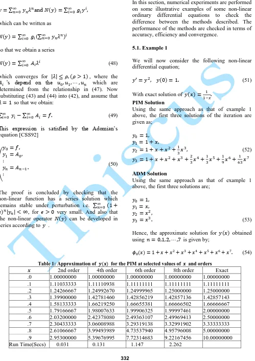
Hence, the approximate solution for obtained using is given by;
(54)
Table 1: Approximation of for the PIM at selected values of and orders
2nd order 4th order 6th order 8th order Exact
Table 2: Approximation of for the ADM at selected values of and orders
2nd order 4th order 6th order 8th order Exact
.0 1.00000000 1.00000000 1.00000000 1.00000000 1.00000000 .1 1.11000000 1.11110000 1.11111100 1.11111111 1.11111111 .2 1.24000000 1.24960000 1.24998400 1.25000000 1.25000000 .3 1.39000000 1.42510000 1.42825900 1.42854331 1.42857143 .4 1.56000000 1.64960000 1.66393600 1.66622976 1.66666667 .5 1.75000000 1.93750000 1.98437500 1.99609375 2.00000000 .6 1.96000000 2.30560000 2.43001600 2.47480576 2.50000000 .7 2.19000000 2.77310000 3.05881900 3.19882131 3.33333333 .8 2.44000000 3.36160000 3.95142400 4.32891136 5.00000000 .9 2.71000000 4.09510000 5.21703100 6.12579511 10.00000000 Run Time (Secs) 0.017 0.032 0.32 0.044
Table 3: Error Estimation of using PIM for selected values of and orders
2nd order 4th order 6th order 8th order .0 0.00000000 0.00000000 0.00000000 0.00000000 .1 0.00077778 0.00000173 0.00000000 0.00000000 .2 0.00733333 0.00007330 0.00000035 0.00000000 .3 0.02957143 0.00075682 0.00000924 0.00000007 .4 0.08533333 0.00447416 0.00011286 0.00000165 .5 0.20833333 0.01992367 0.00093675 0.00002539 .6 0.46800000 0.07621920 0.00636893 0.00030587 .7 1.02900000 0.27324345 0.04014196 0.00341431 .8 2.38933333 1.00506011 0.26462060 0.04203992 .9 7.04700000 4.60323005 2.27685317 0.77832544
Table 4: Error Estimation of using ADM for the selected values of and orders
2nd order 4th order 6th order 8th order .0 0.00000000 0.00000000 0.00000000 0.00000000 .1 0.00111111 0.00001111 0.00000011 0.00000000 .2 0.01000000 0.0004000 0.00001600 0.00000064 .3 0.03857143 0.00347143 0.00031243 0.00002812 .4 0.10666667 0.01706667 0.00273067 0.00043691 .5 0.25000000 0.06250000 0.01562500 0.00390625 .6 0.54000000 0.19440000 0.06998400 0.02519424 .7 1.14333333 0.56023333 0.27451433 0.13451202 .8 2.56000000 1.63840000 1.04857600 0.67108864 .9 7.29000000 5.90490000 4.78296900 3.87420489
Figure 1: Approximation of for the ADM, PIM
and the Exact Solution at the selected values of considering the 8th order
converges slower to the exact solutions. When comparing between the two methods using figure 1, we can see that the PIM is more accurate and converges to the exact solutions faster than the ADM, but the ADM is more efficient than the PIM since the run time estimate for the PIM is much more greater than that of the ADM.
5.2. Example 2
Let’s consider the following non-linear differential equation.
(55)
With exact solution of
.
PIM Solution
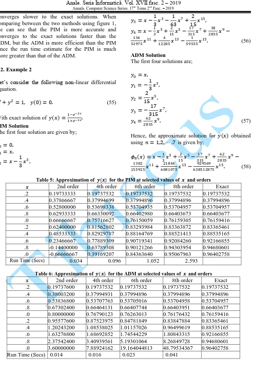
The first four solution are given by;
(56)
ADM Solution
The first four solutions are;
(57)
Hence, the approximate solution for obtained using is given by;
(58)
Table 5: Approximation of for the PIM at selected values of and orders
2nd order 4th order 6th order 8th order Exact
.2 0.19733333 0.19737532 0.19737532 0.19737532 0.19737532 .4 0.37866667 0.37994699 0.37994896 0.37994896 0.37994896 .6 0.52800000 0.53698338 0.53704935 0.53704957 0.53704957 .8 0.62933333 0.66330092 0.66402980 0.66403673 0.66403677 .0 0.66666667 0.75716627 0.76150059 0.76159305 0.76159416 .2 0.62400000 0.81562802 0.83293984 0.83363872 0.83365461 .4 0.48533333 0.82929787 0.88164769 0.88521413 0.88535165 .6 0.23466667 0.77889309 0.90719341 0.92084260 0.92166855 .8 -0.14400000 0.63789308 0.90121266 0.94303954 0.94680601 .0 -0.66666667 0.39169207 0.84363640 0.95067963 0.96402758 Run Time (Secs) 0.034 0.096 1.052 2.593
Table 6: Approximation of for the ADM at selected values of and orders
2nd order 4th order 6th order 8th order Exact
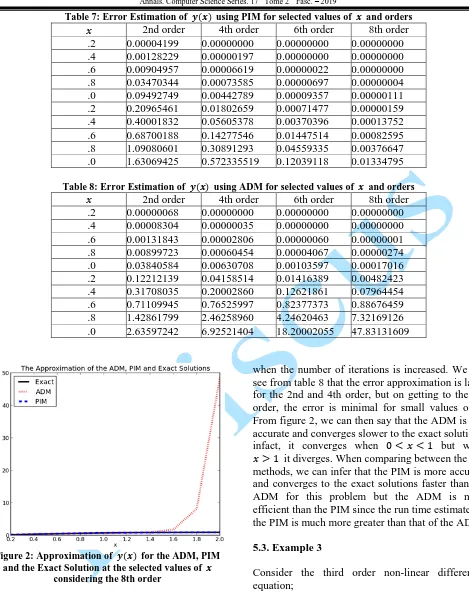
Table 7: Error Estimation of using PIM for selected values of and orders
2nd order 4th order 6th order 8th order .2 0.00004199 0.00000000 0.00000000 0.00000000 .4 0.00128229 0.00000197 0.00000000 0.00000000 .6 0.00904957 0.00006619 0.00000022 0.00000000 .8 0.03470344 0.00073585 0.00000697 0.00000004 .0 0.09492749 0.00442789 0.00009357 0.00000111 .2 0.20965461 0.01802659 0.00071477 0.00000159 .4 0.40001832 0.05605378 0.00370396 0.00013752 .6 0.68700188 0.14277546 0.01447514 0.00082595 .8 1.09080601 0.30891293 0.04559335 0.00376647 .0 1.63069425 0.572335519 0.12039118 0.01334795
Table 8: Error Estimation of using ADM for selected values of and orders
2nd order 4th order 6th order 8th order .2 0.00000068 0.00000000 0.00000000 0.00000000 .4 0.00008304 0.00000035 0.00000000 0.00000000 .6 0.00131843 0.00002806 0.00000060 0.00000001 .8 0.00899723 0.00060454 0.00004067 0.00000274 .0 0.03840584 0.00630708 0.00103597 0.00017016 .2 0.12212139 0.04158514 0.01416389 0.00482423 .4 0.31708035 0.20002860 0.12621861 0.07964454 .6 0.71109945 0.76525997 0.82377373 0.88676459 .8 1.42861799 2.46258960 4.24620463 7.32169126 .0 2.63597242 6.92521404 18.20002055 47.83131609
Figure 2: Approximation of for the ADM, PIM
and the Exact Solution at the selected values of considering the 8th order
Tables 5 and 6 shows the comparison between results of the PIM, ADM and the exact solutions computed for different orders and some selected values of and their run times. The absolute error between the PIM and the exact solutions; the ADM and the exact solutions are shown in tables 7 and 8 respectively. Figure 2 shows the comparison between the PIM, ADM and the exact solutions at the 8th order. From table 7, we can see that the error rate are minimal for small values of , accuracy and convergence of the PIM results generally increases
when the number of iterations is increased. We can see from table 8 that the error approximation is large for the 2nd and 4th order, but on getting to the 8th order, the error is minimal for small values of . From figure 2, we can then say that the ADM is less accurate and converges slower to the exact solutions, infact, it converges when but when it diverges. When comparing between the two methods, we can infer that the PIM is more accurate and converges to the exact solutions faster than the ADM for this problem but the ADM is more efficient than the PIM since the run time estimate for the PIM is much more greater than that of the ADM.
5.3. Example 3
Consider the third order non-linear differential equation;
(59)
With exact solution of . PIM Solution
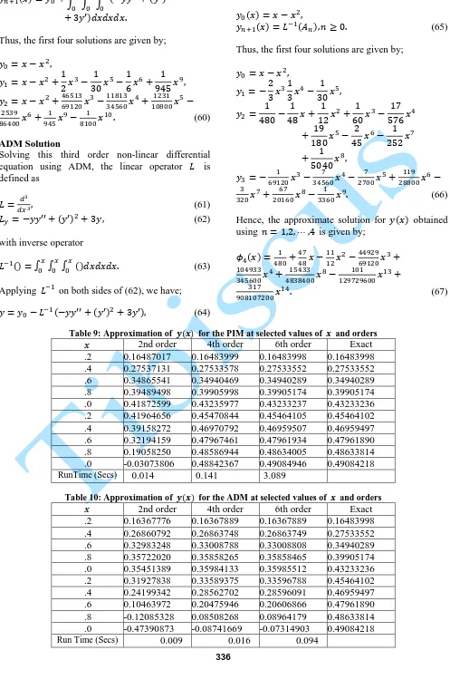
Solving this third order equation, the PIM iterates are obtained by;
Thus, the first four solutions are given by;
(60)
ADM Solution
Solving this third order non-linear differential equation using ADM, the linear operator is defined as
(61)
(62) with inverse operator
(63)
Applying on both sides of (62), we have; (64)
and we obtain the following recurrence relation:
(65)
Thus, the first four solutions are given by;
(66)
Hence, the approximate solution for obtained using is given by;
(67)
Table 9: Approximation of for the PIM at selected values of and orders
2nd order 4th order 6th order Exact
.2 0.16487017 0.16483999 0.16483998 0.16483998 .4 0.27537131 0.27533578 0.27533552 0.27533552 .6 0.34865541 0.34940469 0.34940289 0.34940289 .8 0.39489498 0.39905998 0.39905174 0.39905174 .0 0.41872599 0.43235977 0.43233237 0.43233236 .2 0.41964656 0.45470844 0.45464105 0.45464102 .4 0.39158272 0.46970792 0.46959507 0.46959497 .6 0.32194159 0.47967461 0.47961934 0.47961890 .8 0.19058250 0.48586944 0.48634005 0.48633814 .0 -0.03073806 0.48842367 0.49084946 0.49084218 RunTime (Secs) 0.014 0.141 3.089
Table 10: Approximation of for the ADM at selected values of and orders
2nd order 4th order 6th order Exact
Table 11: Error Estimation of using PIM for selected values of and orders
2nd order 4th order 6th order .2 0.00003019 0.00000001 0.00000000 .4 0.00003579 0.00000026 0.00000000 .6 0.00074748 0.00000180 0.00000000 .8 0.00415676 0.00000824 0.00000000 .0 0.01360637 0.00002742 0.00000001 .2 0.03499446 0.00006742 0.00000003 .4 0.07801225 0.00011295 0.00000010 .6 0.15767731 0.00005571 0.00000044 .8 0.29575564 0.00046870 0.00000191 .0 0.502158024 0.00241851 0.00000728
Table 12: Error Estimation of using ADM for selected values of and orders
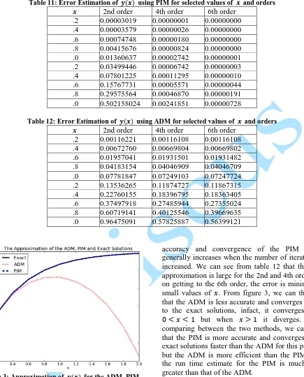
2nd order 4th order 6th order .2 0.00116221 0.00116108 0.00116108 .4 0.00672760 0.00669804 0.00669802 .6 0.01957041 0.01931501 0.01931482 .8 0.04183154 0.04046909 0.04046709 .0 0.07781847 0.07249103 0.07247724 .2 0.13536265 0.11874727 0.11867315 .4 0.22760155 0.18396795 0.18363405 .6 0.37497918 0.27485944 0.27355024 .8 0.60719141 0.40125546 0.39669635 .0 0.96475091 0.57825887 0.56399121
Figure 3: Approximation of for the ADM, PIM
and the Exact Solution at the selected values of considering the 6th order
Tables 9 and 10 shows the comparison between results of the PIM, ADM and the exact solutions computed for different orders and some selected values of and their run times. The absolute error between the PIM and the exact solutions; the ADM and the exact solutions are shown in tables 11 and 12 respectively. Figure 3 shows the comparison between the PIM, ADM and the exact solutions at the 8th order. From table 11, we can see that the error rate are minimal for small values of ,
accuracy and convergence of the PIM results generally increases when the number of iterations is increased. We can see from table 12 that the error approximation is large for the 2nd and 4th order, but on getting to the 6th order, the error is minimal for small values of . From figure 3, we can then say that the ADM is less accurate and converges slower to the exact solutions, infact, it converges when but when it diverges. When comparing between the two methods, we can infer that the PIM is more accurate and converges to the exact solutions faster than the ADM for this problem but the ADM is more efficient than the PIM since the run time estimate for the PIM is much more greater than that of the ADM.
ACKNOWLEDGMENT
The authors are grateful to the reviewers and the handling editor for their helpful comments and suggestions that had greatly improved this work.
REFERENCES
[Abd08] A. H. M. Abdelrazec – Adomian decomposition method: convergence
analysis and numerical
approximations, M.Sc. Thesis,
Ontario, 2008.
[Ado88] G. Adomian – A review of the
decomposition in applied mathematics,
Mathematical analysis and applications, Vol. 135, pp. 501-544, 1988.
[Ado92] G. Adomian – A review of the decomposition method and some recent
results for nonlinear equation,
Mathematical Computational Model., Vol. 13(7), 1992.
[AR96] G. Adomian, R. Rach – Modified
Adomian Polynomials, Mathematical
Computational Model., Vol. 24, No. 11, pp. 39-46, 1996.
[CL55] Coddington E. A., Levinson N. –
Theory of Ordinary Differential
Equations. New York:McGraw-Hill,
1955.
[CSS92] Y. Cherruault, G. Saccomandi, B.
Some – New results for convergence of
Adomian’s method applied to integral
equations, Mathematical computational
modelling, Vol. 16, No. 2, pp. 85-93, 1992.
[G+12] B. Gbadamosi,O. Adebimpe, E. I. Akinola, I. A. Olopade – Soliving
Riccati Equation Using Adomian
Decomposition Method, International
Journal of Pure and Applied Mathematics, Vol. 78, No. 3, pp. 409-417, 2012.
[Lin94] E. Lindelof – Sur l'application de la
méthode des approximations
successives aux équations
différentielles ordinaires du premier
ordre. Comptes rendus hebdomadaires
des séances de l'Académie des sciences. 116: 454-457, 1894.
[MS12] S. S. Motsa, S. Shateyi – New Analytic Solution to the Lane-Emden Equation
of Index 2, Mathematical problems in
Engineering, pp. 1-20, 2012.
[NSS04] R. K. Nagle, E. B. Saff, A. D. Snider – Fundamentals of differential equations
and boundary value problems, 4th