https://doi.org/10.5194/gmd-12-33-2019
© Author(s) 2019. This work is distributed under the Creative Commons Attribution 4.0 License.
Ensemble forecasts of air quality in eastern China – Part 1: Model
description and implementation of the MarcoPolo–Panda prediction
system, version 1
Guy P. Brasseur1,2, Ying Xie3, Anna Katinka Petersen1, Idir Bouarar1, Johannes Flemming4, Michael Gauss5, Fei Jiang6, Rostislav Kouznetsov7, Richard Kranenburg8, Bas Mijling9, Vincent-Henri Peuch4, Matthieu Pommier5, Arjo Segers8, Mikhail Sofiev7, Renske Timmermans8, Ronald van der A10, Stacy Walters2, Jianming Xu3, and Guangqiang Zhou3
1Max Planck Institute for Meteorology, Hamburg, Germany 2National Center for Atmospheric Research, Boulder, CO, USA 3Shanghai Meteorological Service, Shanghai, China
4European Centre for Medium-Range Weather Forecasts, Reading, UK 5Norwegian Meteorological Institute, Oslo, Norway
6Nanjing University, Nanjing, China
7Finnish Meteorological Institute, Helsinki, Finland 8TNO, Utrecht, the Netherlands
9Royal Netherlands Meteorological Institute (KNMI), De Bilt, the Netherlands 10Nanjing University of Information Science and Technology, Nanjing, China
Correspondence:Guy P. Brasseur ([email protected]) Received: 12 June 2018 – Discussion started: 12 July 2018
Revised: 12 October 2018 – Accepted: 31 October 2018 – Published: 3 January 2019
Abstract.An operational multi-model forecasting system for air quality including nine different chemical transport models has been developed and provides daily forecasts of ozone, ni-trogen oxides, and particulate matter for the 37 largest urban areas of China (population higher than 3 million in 2010). These individual forecasts as well as the mean and median concentrations for the next 3 days are displayed on a publicly accessible website (http://www.marcopolo-panda.eu, last ac-cess: 7 December 2018). The paper describes the forecasting system and shows some selected illustrative examples of air quality predictions. It presents an intercomparison of the dif-ferent forecasts performed during a given period of time (1– 15 March 2017) and highlights recurrent differences between the model output as well as systematic biases that appear in the median concentration values. Pathways to improve the forecasts by the multi-model system are suggested.
1 Introduction
The rapid economic growth in China has been accompanied by a substantial degradation of air quality, particularly in the densely populated areas of the eastern part of the country. Air pollution is the source of cardiovascular and respiratory illness, increased stress to heart and lungs, and cell damage in the respiratory system, which in turn can result in fatali-ties resulting from ischemic heart disease, chronic obstruc-tive pulmonary disease (COPD – please refer to Appendix A for a list of other abbreviations and their definitions), and lower respiratory infections. To address this problem, China is taking effective measures to reduce the emission of pri-mary pollutants such as nitrogen oxides (NOx), volatile
of predicted events. The implementation of such measures requires that accurate forecasts of air quality be produced and made available to local and regional authorities. Alerts to warn the public of the imminence of acute pollution episodes can be released several days before the event on the basis of model predictions.
Advanced forecast models include a detailed formulation of the chemical and physical processes responsible for the formation of secondary pollutants such as ozone and partic-ulate matter in response to the emissions of primary species produced as a result of industrial, agricultural, and residen-tial activities, energy production, and transportation. These models simulate the transport of these constituents by the at-mospheric circulation as well as vertical exchanges by con-vective motions and turbulent boundary layer mixing. Mete-orological information provided by weather forecast models is therefore an essential input to regional air quality models. Surface deposition of oxidized compounds and wet scaveng-ing of soluble species are also taken into account. The atmo-spheric concentrations of the chemical and physically inter-acting species are obtained by solving a mathematically stiff system of partial differential equations with appropriate ini-tial and boundary conditions.
The approach used to produce predictions of air quality bears a lot of resemblance to the methods used for weather forecasts. In both cases, models make use of similar numer-ical algorithms, assimilate data, and produce large amounts of output that have to be analyzed and evaluated, and even-tually disseminated to the public in the form of easily ac-cessible information. The steady progress made in the nu-merical weather prediction since the 1980s (Bauer et al., 2015), through combined scientific, computational, and ob-servational advances, has also considerably improved our ca-pability of providing predictive information on air quality and on its impacts for human society (i.e., health, food pro-duction, and the state of ecosystems).
Many models are available for operationally forecasting air quality (Kukkonen et al., 2012) and have been tested in different contexts. These models are usually driven by differ-ent input data (surface emissions, weather forecasts, chem-ical schemes, aerosol formulation, land-use data, boundary conditions, etc.) and hence generate different output (e.g., different concentrations of chemical species). In most cases, it is difficult to clearly distinguish between models that per-form well and models that perper-form poorly because the suc-cess of individual models varies with the conditions that are encountered (e.g., geographic location, season, meteorologi-cal situation) and can be different for the different chemimeteorologi-cal species and for different statistical parameters. If the mod-els involved have been developed fairly independently from each other their results can be combined and their individ-ual behaviors can be examined by comparing the predicted fields to the median or the mean derived from the ensem-ble of simulations. Much can be learned from a systematic
day-by-day examination of the model behavior operated in a forecast mode.
Building an ensemble of models is an attractive approach to forecast air quality because the inter-model variability pro-vides insight on the robustness of the results or conversely on their uncertainties (McKeen et al., 2005; Vautard et al., 2006; Solazzo et al., 2012). Further, the composite products have usually better overall performance than the results produced by individual systems (McKeen et al., 2005; Galmarini et al., 2013; Riccio et al., 2007; Sofiev et al., 2015, 2017). This ap-proach is especially useful in the context of decision-making since it samples the uncertainty space associated with the dif-ferent individual forecasts.
A numerical weather forecast is usually based on a single model ensemble in which the initial conditions are slightly perturbed so that different likely evolutions of the atmo-spheric dynamics can be projected. In the case of air qual-ity forecasts, which are not only initial-value problems, it is advisable to also perturb emissions, meteorology, and bound-ary conditions as well as model parameters (kinetic reaction rates, etc.), which is best performed by considering a multi-model ensemble (Dabberdt and Miller, 2000). Nevertheless, in addition, it would also be useful to assess the behavior of a single air quality model, which shows is driven by different realizations of ensemble meteorological forecasts, different emission scenarios, and different chemical schemes.
The models used in the present study have been developed fairly independently, and this leads to a rather broad range of model results. Model performance does not only depend on the quality of emissions datasets: they differ for a wide range of reasons, including dynamical and weather aspects but also the adopted formulation (e.g., parameterizations, op-erator splitting, time integration) and numerical algorithms. An inspection of the different choices made in the models can lead to some improvements in model configurations and hence will reduce the “artificial” spread between calculated fields. This spread often results from errors in the configu-ration (e.g., setup bugs) or from inaccuracies in the adopted input parameters (e.g., land use). By including each model configuration within a large ensemble, the combined perfor-mance of the forecast system is considerably less affected by initial implementation issues or an inadequate choice of input parameters applied in individual models.
2018) discusses in more detail the performance of the fore-cast system including the representativeness of the model-observation discrepancies, specifically in urban areas. Ap-proaches to improve the performance of the system are pre-sented in Sect. 5.
The ensemble of models considered in the present study has been assembled under the Panda and MarcoPolo projects supported by the European Commission within the Frame-work Programme 7 (FP7). Seven models were initially included in the operational system: the global IFS (In-tegrated Forecasting System) model developed and oper-ated by the European Centre for Medium-Range Weather Forecasts (ECMWF), five regional models implemented by European research and service institutions (CHIMERE by the Royal Netherlands Meteorological Institute (KNMI), Weather Research and Forecasting model coupled to chem-istry by the Max Planck Institute for Meteorology (WRF-Chem-MPIM), SILAM (System for Integrated Modeling of Atmospheric Composition) by the Finnish Meteorolog-ical Institute (FMI), EMEP/MSC-W (European Monitor-ing and Evaluation Programme/Meteorological Synthesiz-ing Centre-West Model hosted at the Norwegian Meteo-rological Institute) by the Norwegian MeteoMeteo-rological In-stitute (MET.Norway), LOTOS-EUROS (Long-term Ozone Simulations – European Operational Smog) by The Nether-lands Organisation for Applied Scientific Research (TNO)), and one model (WRF-Chem-SMS) applied in China by the Shanghai Meteorological Service (SMS). In later steps, forecasts by additional regional models applied by Nanjing University (WRF–CMAQ; CMAQ – Community Multiscale Air Quality) and by the Shanghai Meteorological Service (WARMS-CMAQ; WARMS – WRF ADAS Real-time Mod-eling System (WARMS)) were added to the ensemble. In the following section, we provide a brief overview of these dif-ferent models. Only seven of them contribute to the inter-comparison presented in Sect. 4.
2 Description of the models included in the ensemble In the following subsections, each of the nine participating models will be described. Table 2a–b present the key charac-teristics of each model involved in the intercomparison, and Table 3 summarizes the emissions adopted in each model. 2.1 IFS
IFS is ECMWF’s global numerical weather prediction sys-tem. As part of the past series of European projects MACC and now of CAMS, IFS has been developed to represent op-tionally chemical processes in the troposphere and in the stratosphere. Flemming et al. (2015) provide a detailed de-scription of the modeling of chemical processes in the IFS, and Inness et al. (2015) describe the data assimilation as-pects.
For the work presented here, the version of IFS used is Cycle 43R1 (see documentation at https: //www.ecmwf.int/en/forecasts/documentation-and-support/ changes-ecmwf-model/ifs-documentation, last access: 7 De-cember 2018). The model is run globally at a resolution of T511 (about 40 km) on the horizontal and with 60 levels on the vertical extending up to the top of the stratosphere. The chemical package used originates from the TM5 chemistry and transport model (Huijnen et al., 2010). It has been fully integrated into the IFS code and comprises 54 tracers and 120 reactions focusing on tropospheric-ozone–CO– NMVOC–NOx chemistry. In the configuration used here,
stratospheric ozone is modeled with a simple linearized scheme. Aerosols are represented using the scheme de-scribed by Morcrette et al. (2009), which includes five species: dust, sea salt, black carbon, organic carbon, and sulfates. Tracers are transported using the semi-Lagrangian scheme available in IFS with a mass fixer activated in order to minimize mass nonconservation.
During the study period, IFS has been run twice daily (5-day forecasts) assimilating a range of satellite chemical data on top of the full list of meteorological satellite and non-satellite data that ECMWF uses for its medium-range weather forecasts. Table 1 indicates the satellite data streams actively assimilated for the experiments presented here. As a result, IFS forecasts benefit from all these observations to afford a realistic representation of large scales for weather parameters as well as, to some extent, for chemical variables (species assimilated).
IFS used the MACCity emission dataset updated for the year 2017. Biogenic emissions of volatile organic com-pounds (VOCs) were taken from a climatology of a multi-year Model of Emissions of Gases and Aerosols from Na-ture (MEGAN) simulation. Daily emissions from biomass burning were derived from satellite retrieval of fire radiative power (FRP) from the MODIS instruments by the Global Fire Assimilation System (GFAS; Kaiser et al., 2012). The observed fire emissions from the day before the forecast start are used for all 5 days of the forecast. Desert dust and sea salt emissions were simulated online for each time step based on the IFS meteorological fields and the land use.
Table 1.Satellite data streams (atmospheric composition variables only) assimilated in IFS.
Instrument Satellite Space agency Data provider Species
MODIS EOS-Aqua, EOS-Terra NASA NASA AOD
MLS EOS-Aura NASA O3profile
OMI EOS-Aura NASA KNMI O3, NO2, SO2
SBUV-2 NOAA-19 NOAA NOAA O3profile
IASI METOP-A, METOP-B EUMETSAT/CNES ULB/LATMOS CO
MOPITT EOS-Terra NASA NCAR CO
GOME-2 METOP-A, METOP-B EUMETSAT/ESA AC-SAF O3, SO2
OMPS Suomi-NPP NOAA EUMETSAT O3
PMAp METOP-A, METOP-B EUMETSAT EUMETSAT AOD
2.2 CHIMERE
CHIMERE is a regional chemistry transport model used for analysis, scenarios, and forecast (Menut et al., 2013a). When used in the forecast mode, the model provides local-scale information (to be compared with data from numerous air quality networks) or regional-scale information (e.g., the French PREV’AIR and the CAMS systems). CHIMERE is an open-source model, freely distributed at http://www.lmd. polytechnique.fr/chimere/ (last access: 7 December 2018). In this version, CHIMERE is used in off-line mode at a spa-tial resolution of 0.25◦ (about 25 km). It is forced by pre-calculated hourly meteorological fields for the dynamics and by several emissions fluxes for the chemistry. The emis-sions are pre-calculated or online estimated in the model with anthropogenic emissions (MEIC 2010), biogenic emissions with the online MEGAN (Guenther et al., 2006), mineral dust (Menut et al., 2013b), and biomass burning emissions (Tur-quety et al., 2014). The gas-phase chemistry is calculated us-ing the MELCHIOR2 mechanism, and the aerosols are rep-resented using a distribution of 10 bins, from 40 nm to 40 µm to describe both number and mass well. The chemical bound-ary conditions are provided by the LMDz-INCA model for gas and particles (Szopa et al., 2009), except for mineral dust, which is extracted from global GOCART simulations (Ginoux et al., 2001). Further information about the imple-mentation of the model for air quality forecasts in China can be obtained from Ronald van der A ([email protected]) at KNMI and on the website http://www.lmd.polytechnique.fr/ chimere/CW-download.php (last access: 7 December 2018).
2.3 WRF-Chem-MPIM
WRF-Chem is a mesoscale non-hydrostatic meteorological model (Skamarock et al., 2008) coupled “online” with chem-istry that simultaneously predicts meteorological and chemi-cal components of the atmosphere (Grell et al., 2005; Fast et al., 2006).
The model version used at the Max Planck Institute for Meteorology (MPIM), WRF-Chem-MPIM, is based on ver-sion 3.6.1 of the WRF-Chem model coupled to the
gas-phase chemistry and the aerosol microphysics schemes pro-vided by the Model for Ozone and Related Chemical Tracers (MOZART-4; Emmons et al., 2010) and the Model for Sim-ulating Aerosol Interactions and Chemistry (MOSAIC; Za-veri et al., 2008), respectively. Aerosol sizes are represented by four consecutive bins, and the formation of secondary or-ganic aerosol (SOA) from anthropogenic precursors is pa-rameterized according to Hodzic and Jimenez (2011).
Two nested model domains with horizontal resolutions of 60 km (Asian continent from India to Japan) and 20 km (eastern China), respectively, are implemented. The ver-tical grid is composed of 51 levels extending from the surface to 10 hPa (∼30 km). A more complete descrip-tion of the selected physical and chemical opdescrip-tions is pro-vided in the WRF and in the WRF-Chem user’s guides un-der http://www2.mmm.ucar.edu/wrf/users/docs/user_guide_ V3.6/ARWUsersGuideV3.6.1.pdf (last access: 7 Decem-ber 2018) and https://ruc.noaa.gov/wrf/wrf-chem/Users_ guide.pdf (last access: 7 December 2018).
The WRF-Chem-MPIM model forecasts are initialized and forced at the lateral boundaries every day by 6-hourly meteorological analysis data from the NCEP Global Fore-cast System (GFS) at 0.5◦ resolution. For the chemical and aerosol species, 6-hourly datasets are provided by the global operational forecasting system implemented within the Copernicus Atmospheric Monitoring Service project (Flemming et al., 2015). More information on the model’s configuration can be obtained from Idir Bouarar ([email protected]) at the Max Planck Institute for Meteorology and on the website http://www2.mmm. ucar.edu/wrf/users/downloads.html (last access: 7 Decem-ber 2018).
2.4 SILAM
and Sofiev (2012). The surface resistance model for gases is based on a modified Wesely scheme (Wesely, 1989).
The gas-phase chemistry was simulated with CBM-IV, with reaction rates updated according to the recommenda-tions of IUPAC (http://iupac.pole-ether.fr, last access: 7 De-cember 2018) and JPL (http://jpldataeval.jpl.nasa.gov, last access: 7 December 2018) and the terpenes oxidation added from the 2005 Carbon Bond (CB05) chemical mechanism re-action list (Yarwood et al., 2005). The sulfur chemistry and secondary inorganic aerosol formation is computed with an updated version of the DMAT scheme (Sofiev, 2000), and secondary organic aerosol formation is computed with the volatility basis set (VBS; Donahue et al., 2006), with the volatility distribution of anthropogenic organic carbon (OC) taken from Shrivastava et al. (2011).
The MACCity land-based emissions are used to-gether with the Ship Traffic Emission Assessment Model (STEAM). The simulations include sea salt emissions as in Sofiev et al. (2011), biogenic VOC emissions as in Poup-kou et al. (2010), wild land fire emissions as in Soares et al. (2015), and desert dust.
The grid cell size was roughly 15 km×10 km (0.125◦×0.125◦) covering the whole of China, India, Japan, and several countries of Southeast Asia (7◦N, 67◦E) – (54◦N, 147◦E). The Asian forecasts are nested into the SILAM global air quality forecasts (http://silam.fmi.fi, last access: 7 December 2018), from where they take lateral and top boundary conditions. The initial conditions for each run are taken from the previous day’s forecast or, in case of failure, from global computations. Detailed information about the SILAM modeling system can be obtained from Mikhail Sofiev ([email protected]) and from Rostislav Kouznetsov ([email protected]) and on the website of the Finnish Meteorological Institute (http://silam.fmi.fi/).
2.5 EMEP
EMEP/MSC-W (hereafter referred to as “EMEP model”) is a 3-D Eulerian chemical transport model described in detail in Simpson et al. (2012). Although the model has tradition-ally been aimed at European simulations, global modeling has been possible for many years (Jonson et al., 2010; Wild et al., 2012). The EMEP configuration for the present study covers the east Asian domain (15–55◦N×90–135◦E) with a horizontal resolution of 0.1◦×0.1◦(longitude–latitude). The model uses 20 vertical levels defined as sigma coordinates. The 10 lowest levels are within the planetary boundary layer (PBL), and the top of the model domain is at 100 hPa.
Particulate matter (PM) emissions are split into elementary carbon, organic matter (OM) (here assumed inert), and the remainder, for both fine and coarse PM. The OM emissions are further divided into fossil fuel and wood-burning com-pounds for each source sector. As in Bergström et al. (2012), the OM / OC ratio of emissions by mass is assumed to be
1.3 for fossil-fuel sources and 1.7 for wood-burning sources. The model also calculates windblown dust emissions from soil erosion. Secondary PM2.5aerosol consists of inorganic
sulfate, nitrate, ammonium, and SOA; the latter is gener-ated from both anthropogenic and biogenic emissions (an-thropogenic SOA and biogenic SOA, respectively), using the VBS scheme detailed in Bergström et al. (2012) and Simpson et al. (2012).
Model updates since Simpson et al. (2012), resulting in EMEP model version rv4.9 as used here, have been de-scribed in Simpson et al. (2016) and references cited therein. The main changes concern a new calculation of aerosol surface area, revised parameterizations of N2O5 hydrolysis
on aerosols, additional gas-aerosol loss processes for O3,
HNO3, and HO2, a new scheme for ship NOxemissions, and
the use of new maps for global leaf area (used to calculate biogenic VOC emissions) – see Simpson et al. (2015) for de-tails. The EMEP model, including a user guide, is publicly available as open-source code at https://github.com/metno/ emep-ctm (last access: 7 December 2018). For more details, please contact Michael Gauss ([email protected]).
The EMEP forecasts are driven by 3-hourly meteorologi-cal forecast data from the ECMWF IFS model at 0.1◦ resolu-tion. As for WRF-Chem, 6-hourly datasets for the chemical and aerosol species are provided by the global operational forecasting system implemented within the Copernicus At-mospheric Monitoring Service project.
2.6 LOTOS-EUROS
LOTOS-EUROS is a three-dimensional regional chemistry transport model for simulation of trace gases and aerosol concentrations in the boundary layer. Meteorological input is obtained from an off-line model, in this study from ECMWF. The model is of intermediate complexity allowing long-term model simulations. For a detailed model description, we refer to Manders et al. (2017) and references therein.
In this study LOTOS-EUROS version 1.10 was used to simulate air quality over China. The configuration is de-scribed by Timmermans et al. (2017), who adopted this ver-sion of the model to investigate the origin of fine particu-late matter across China using a source apportionment tech-nique. Through a one-way nesting procedure a simulation over east China was performed on a resolution of 0.25◦ longi-tude by 0.125◦latitude, approximately 21 km by 15 km. This domain is nested in a larger domain covering China almost entirely with a resolution of 1◦ longitude by 0.5◦ latitude,
the model, and is here taken from the meteorological input. More details about the code can be obtained by contacting Renske Timmermans ([email protected]) at TNO or by consulting the website https://lotos-euros.tno.nl/ (last access: 7 December 2018).
2.7 WRF-Chem-SMS
WRF-Chem-SMS hosted at the Shanghai Meteorological Service is based on WRF-Chem (Grell et al., 2005) ver-sion 3.2. The Regional Acid Deposition Model verver-sion 2 (RADM2; Chang et al., 1989) is used to represent gas-phase chemistry. ISORROPIA II is implemented to treat thermo-dynamic equilibrium for inorganic aerosols (Fountoukis and Nenes, 2007), and the Secondary ORGanic Aerosol Model (SORGAM) (Schell et al., 2001) is used to parameterize secondary organic aerosol formation. A Madronich TUV scheme is applied for photolysis (Madronich and Flocke, 1999; Tie et al., 2003). The model domain covers the east-ern region of China with horizontal resolutions of 6 km and 28 vertical layers. Biogenic emissions are calculated online using MEGAN (Guenther et al., 2012). The multi-resolution emission inventory for China (MEIC inventory, http://www.meicmodel.org/ (last access: 7 December 2018); Li et al., 2014; Liu et al., 2015) for the year 2010 is used to represent anthropogenic emissions.
The modeling system is initialized and forced at the lateral boundaries every day by 6-hourly data from the NCEP GFS at 0.5◦ resolution. For chemical species, a previous model-ing result is used for initial conditions. MOZART-4 historic data are employed as the gaseous chemical lateral boundary, and a real-time forecast of dust from the WRF-Dust model is employed as a dust lateral boundary every 6 h. More detailed information can be found in Zhou et al. (2017) and by con-tacting Jianming Xu ([email protected]) at the Shanghai Meteorological Service.
2.8 WRF–CMAQ
A regional air quality operational forecasting system was de-veloped at Nanjing University, China, on the basis of the WRF–CMAQ model. The versions adopted for the WRF (Weather and Forecasting) and CMAQ (Community Multi-scale Air Quality) models are V3.5 and V4.7.1, respectively. Two nested domains with horizontal resolutions of 36 and 12 km are adopted for the forecasts. The outer domain cov-ers the entire continental region of China as well as surround-ing countries in east Asia. The inner domain mainly focuses on the densely populated area of eastern China. The num-ber of grid points adopted for the WRF model are 170×130 and 202×226, respectively with 51σ layers in the vertical (12 layers below 1.5 km a.g.l.) between the surface and the model top at 50 hPa. The CMAQ model is applied to the same domains but with three grid cells removed at each lat-eral boundary of the WRF domains. Ovlat-erall, 15 vertical
lay-ers are selected from the 51 WRF laylay-ers, including about 8 layers in the boundary layer and 7 layers in the free tropo-sphere.
Anthropogenic emissions are supplied off-line from the MIX inventory (Li et al., 2017). Terrestrial biogenic emis-sions are calculated off-line using MEGAN v2.04 (Guen-ther et al., 2006). Sea salt emissions are incorporated into the AERO4 aerosol module and calculated online in CMAQ. Windblown dust is derived online from the WRF-Dust model. Open biomass burning emissions are not considered here. It should be noted that the anthropogenic emissions are not fixed in this system but are automatically adjusted every week according to the system performance in the past week. The adopted scaling factors are determined from the devia-tion between the weekly averaged calculated and observed concentrations of SO2, NOx, CO, PM2.5, and PM10 in 334
Chinese prefectures.
The system provides a forecast every day for the next 192 h. The NCEP GFS’s products at 00:00 UTC are used for the initial and boundary conditions of the WRF model with a resolution of 0.5◦ and with a 3 h interval. For the CMAQ model, the boundary conditions are created using ideal profiles, and the chemical initial fields are initialized from the previous forecasting. In addition, hourly averaged observed concentrations of SO2, NO2, CO, O3, PM2.5, and
PM10from 1415 national control air-quality-monitoring sites
are assimilated into the initial fields using an optimal inter-polation method (Lorenc, 1981). More information on the code can be obtained from Fei Jiang ([email protected]) at Nanjing University. Information on WRF–CMAQ is also available on the website http://carbon.nju.edu.cn/cn/ (last access: 7 December 2018) and https://www.epa.gov/cmaq/ cmaq-models-0 (last access: 7 December 2018).
2.9 WARMS-CMAQ
The Community Multiscale Air Quality (CMAQ) model is a 3-D Eulerian chemical transport model that explicitly simu-lates emissions, gas-phase, aqueous, and mixed-phase chem-istry, advection and dispersion, aerosol thermodynamics and physics, and wet and dry deposition. A detailed description and an evaluation of the CMAQ model are available in the papers by Byun and Schere (2006), Foley et al. (2010), and Appel et al. (2017). Several studies have applied the CMAQ model to study the air quality in China. For example, Zheng et al. (2015) used the WRF–CMAQ model to study the im-pact of heterogeneous chemistry during the January 2013 haze episode. Hu et al. (2016) performed a 1-year retrospec-tive simulation using the WRF–CMAQ model to study the O3 and particulate matter formation with a detailed
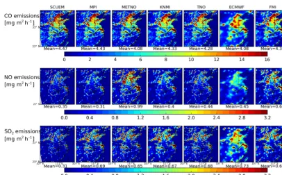
Figure 1.Surface emissions of CO, NO, and SO2(mg m−2h−1) adopted by the different models (average for the period 1–14 March 2017).
Note that the SCUEM emissions are those used in the WRF-Chem-SMS model.
In this version, CMAQ is used in an off-line mode. It is forced by pre-calculated hourly meteorological fields for the dynamics and by several emissions fluxes for the chemistry. Meteorology fields that drive chemical transport are pro-duced by the SMS-WARMS. The SMS-WARMS has been extensively evaluated and provides weather predictions in eastern China. The modeling domain consists of 760 by 600 horizontal grids at 9 km resolution, with 51 layers in the ver-tical. As a subdomain of the SMS-WARMS run, the CMAQ domain consists of 430 by 370 horizontal grid cells at 9 km resolution. In the vertical, 26 layers are applied.
The anthropogenic emissions are based on the monthly HTAP v2 dataset (http://edgar.jrc.ec.europa.eu/htap_v2/, last access: 7 December 2018) (Janssens-Maenhout et al., 2015) for the year 2010. As suggested by operational forecasting results, the HTAP NOx, SO2 emissions are adjusted to
ac-count for rapid economic growth in the region. Biogenic emissions are estimated by MEGAN version 2.10 (Guenther et al., 2012). Currently, dust and biomass burning emissions are not included.
For the SMS-WARMS model forecasts, the NCEP GFS output at 0.5◦ is used as a background for the ADAS data assimilation scheme, which ingests many local observations (e.g., radar and buoys), and to provide lateral boundary conditions. The chemical boundary conditions are currently based on the default vertical profiles of gaseous species and aerosols in CMAQ that represent clean-air conditions. For more details, please contact Ying Xie ([email protected]) at the Shanghai Meteorological Service. The CMAQ code
available on the U.S. EPA modeling site https://github.com/ USEPA/CMAQ/ (last access: 7 December 2018).
3 Adopted emissions
The choice of the adopted surface emissions for primary chemical species has a significant influence on the atmo-spheric concentrations calculated for these species and for re-lated secondary pollutants. In this intercomparison exercise, the different groups involved have adopted their preferred an-thropogenic emissions based on published inventories such as MEIC (Li et al., 2014; Liu et al., 2015), MACCity (Granier et al., 2011), EDGAR (Emission Database for Global Atmo-spheric Research; Muntean et al., 2014; Crippa et al., 2016), and HTAP (Janssens-Maenhout et al., 2015). An inventory developed specifically for the Panda project called PanHam has been obtained by combining information from the MEIC and HTAP inventories. Each model uses its own formula-tion for dust mobilizaformula-tion or seal salt emissions. In most cases, the biogenic emissions are derived online or off-line from MEGAN (Guenther et al., 2006, 2012). Table 3 pro-vides more details about the specified emissions and Fig. 1 shows the mean distribution of the anthropogenic emissions for CO, NO, and SO2 adopted by different models during
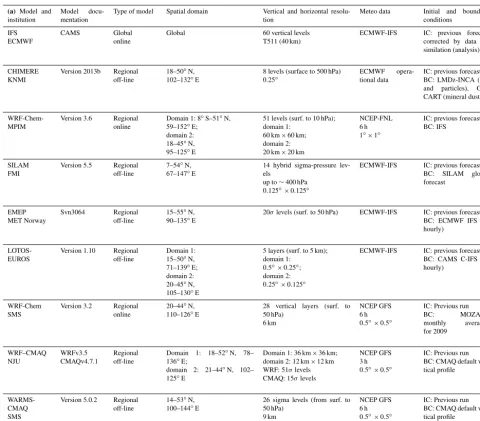
Table 2.Description of the different models.
(a) Model and institution
Model docu-mentation
Type of model Spatial domain Vertical and horizontal resolu-tion
Meteo data Initial and boundary conditions
IFS ECMWF
CAMS Global
online
Global 60 vertical levels
T511 (40 km)
ECMWF-IFS IC: previous forecast corrected by data as-similation (analysis)
CHIMERE KNMI
Version 2013b Regional off-line
18–50◦N, 102–132◦E
8 levels (surface to 500 hPa) 0.25◦
ECMWF
opera-tional data
IC: previous forecast BC: LMDz-INCA (gas and particles), GO-CART (mineral dust)
WRF-Chem-MPIM
Version 3.6 Regional online
Domain 1: 8◦S–51◦N,
59–152◦E; domain 2: 18–45◦N,
95–125◦E
51 levels (surf. to 10 hPa); domain 1:
60 km×60 km; domain 2: 20 km×20 km
NCEP-FNL 6 h 1◦×1◦
IC: previous forecast BC: IFS
SILAM FMI
Version 5.5 Regional off-line
7–54◦N, 67–147◦E
14 hybrid sigma-pressure lev-els
up to∼400 hPa 0.125◦×0.125◦
ECMWF-IFS IC: previous forecast BC: SILAM global forecast
EMEP MET Norway
Svn3064 Regional
off-line
15–55◦N,
90–135◦E
20σlevels (surf. to 50 hPa) ECMWF-IFS IC: previous forecast BC: ECMWF IFS (3-hourly)
LOTOS-EUROS
Version 1.10 Regional off-line
Domain 1: 15–50◦N, 71–139◦E;
domain 2: 20–45◦N, 105–130◦E
5 layers (surf. to 5 km); domain 1:
0.5◦×0.25◦;
domain 2: 0.25◦×0.125◦
ECMWF-IFS IC: previous forecast BC: CAMS C-IFS (3-hourly)
WRF-Chem SMS
Version 3.2 Regional online
20–44◦N,
110–126◦E
28 vertical layers (surf. to 50 hPa)
6 km
NCEP GFS 6 h 0.5◦×0.5◦
IC: Previous run
BC: MOZART monthly averages for 2009 WRF–CMAQ NJU WRFv3.5 CMAQv4.7.1 Regional off-line
Domain 1: 18–52◦N, 78– 136◦E;
domain 2: 21–44◦N, 102–
125◦E
Domain 1: 36 km×36 km; domain 2: 12 km×12 km WRF: 51σlevels CMAQ: 15σlevels
NCEP GFS 3 h 0.5◦
×0.5◦
IC: Previous run BC: CMAQ default ver-tical profile
WARMS-CMAQ SMS
Version 5.0.2 Regional off-line
14–53◦N,
100–144◦E
26 sigma levels (from surf. to 50 hPa)
9 km
NCEP GFS 6 h 0.5◦×0.5◦
IC: Previous run BC: CMAQ default ver-tical profile
(WRF-Chem-MPIM) to 0.99 mg m−2h−1(EMEP) but with values around 0.30–0.45 mg m−2h−1 used by most mod-els. For sulfur dioxide, produced primarily from coal com-bustion, the adopted values range from 0.31 mg m−2h−1 (WRF-Chem-SMS) to 0.73 mg m−2h−1(IFS) but with val-ues around 0.67 mg m−2h−1 adopted in most models. The low values adopted for WRF-Chem-SMS reflect the likely impact of the recent measures taken in China to limit the emissions from coal burning facilities.
Emission inventories that are currently available to the modeling community usually account for anthropogenic emissions for the years 2010 to 2012 and hence do not ac-count for the substantial reduction in the emissions that took place since around 2014 as a result of actions taken by the Chinese authorities. The lower emission values adopted by
several models may therefore be more realistic for providing chemical weather forecasts in 2017.
4 Operational forecasts provided by the MarcoPolo–Panda system
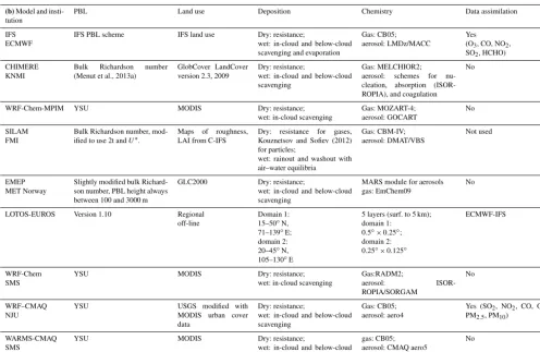
in-Table 2.Continued.
(b)Model and insti-tution
PBL Land use Deposition Chemistry Data assimilation
IFS ECMWF
IFS PBL scheme IFS land use Dry: resistance;
wet: in-cloud and below-cloud scavenging and evaporation
Gas: CB05; aerosol: LMDz/MACC
Yes (O3, CO, NO2,
SO2, HCHO)
CHIMERE KNMI
Bulk Richardson number
(Menut et al., 2013a)
GlobCover LandCover version 2.3, 2009
Dry: resistance;
wet: in-cloud and below-cloud scavenging
Gas: MELCHIOR2; aerosol: schemes for nu-cleation, absorption (ISOR-ROPIA), and coagulation
No
WRF-Chem-MPIM YSU MODIS Dry: resistance;
wet: in-cloud scavenging
Gas: MOZART-4; aerosol: GOCART
No
SILAM FMI
Bulk Richardson number, mod-ified to use 2t andU∗.
Maps of roughness, LAI from C-IFS
Dry: resistance for gases, Kouznetsov and Sofiev (2012) for particles;
wet: rainout and washout with air–water equilibria Gas: CBM-IV; aerosol: DMAT/VBS Not used EMEP MET Norway
Slightly modified bulk Richard-son number, PBL height always between 100 and 3000 m
GLC2000 Dry: resistance;
wet: in-cloud and below-cloud scavenging
MARS module for aerosols gas: EmChem09
No
LOTOS-EUROS Version 1.10 Regional
off-line
Domain 1: 15–50◦N,
71–139◦E;
domain 2: 20–45◦N, 105–130◦E
5 layers (surf. to 5 km); domain 1:
0.5◦×0.25◦;
domain 2: 0.25◦×0.125◦
ECMWF-IFS
WRF-Chem SMS
YSU MODIS Dry: resistance;
wet: in-cloud scavenging
Gas:RADM2; aerosol: ISOR-ROPIA/SORGAM No WRF–CMAQ NJU
YSU USGS modified with
MODIS urban cover
data
Dry: resistance;
wet: in-cloud and below-cloud scavenging
Gas: CB05; aerosol: aero4
Yes (SO2, NO2, CO, O3,
PM2.5, PM10)
WARMS-CMAQ SMS
YSU MODIS Dry: resistance;
wet: in-cloud and below-cloud scavenging
gas: CB05; aerosol: CMAQ aero5
No
dividual models, are posted on a dedicated website (http: //www.marcopolo-panda.eu/, last access: 7 December 2018) and Chinese mirror site (http://116.62.195.108/, last access: 7 December 2018). For the 37 Chinese cities with a popu-lation above 3 million in 2010, the predicted concentration values of ozone, NO2, PM2.5, and PM10 are compared each
hour to local measurements reported by the Chinese monitor-ing network (http://pm25.in/, last access: 7 December 2018). Observations for each city represent the mean of several mea-surements performed within one city (usually 5–12 stations). The data are averaged to city-center coordinates.
We start by presenting a few examples of randomly se-lected forecasts as provided by the MarcoPolo–Panda system to illustrate the diversity among the models and the differ-ences obtained under different situations. The performance of each individual model varies from day to day because it strongly depends on the individual weather forecast (me-teorological situation, cloudiness, precipitation, etc.) that is adopted to simulate transport, photochemistry, and deposi-tion. Therefore, this first description of model forecasts does not provide reliable information on the accuracy of the fore-casts provided by the different models included in the ensem-ble.
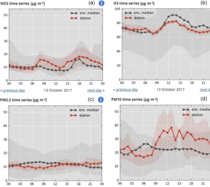
The first example presents a relatively successful forecast made for the coastal city of Xiamen in southeast China on 13 October 2017. The panels in Fig. 3 show the excellent agreement in the case of NO2, ozone, and PM2.5,
suggest-ing that the median values derived from the individual mod-els capture well the features associated with the meteorolog-ical situation, atmospheric transport, and the emissions in the region on that particular day. The situation corresponds to very clean conditions, with PM2.5 and NO2
concentra-tions of the order of 10–15 µg m−3. The predicted ozone con-centration ranges from 70 to 90 µg m−3(35 to 45 ppbv). In-terestingly, however, the predicted PM10 concentrations are
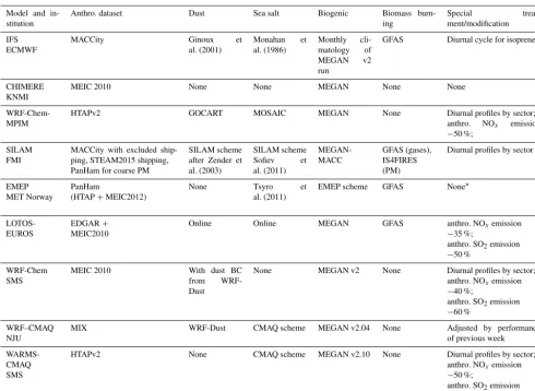
Table 3.Adopted emissions.
Model and in-stitution
Anthro. dataset Dust Sea salt Biogenic Biomass
burn-ing
Special
treat-ment/modification
IFS ECMWF
MACCity Ginoux et
al. (2001) Monahan et al. (1986) Monthly cli-matology of MEGAN v2 run
GFAS Diurnal cycle for isoprene
CHIMERE KNMI
MEIC 2010 None None MEGAN None None
WRF-Chem-MPIM
HTAPv2 GOCART MOSAIC MEGAN None Diurnal profiles by sector;
anthro. NOx emission
−50 %; SILAM
FMI
MACCity with excluded ship-ping, STEAM2015 shipship-ping, PanHam for coarse PM
SILAM scheme after Zender et al. (2003) SILAM scheme Sofiev et al. (2011) MEGAN-MACC GFAS (gases), IS4FIRES (PM)
Diurnal profiles by sector
EMEP MET Norway
PanHam
(HTAP+MEIC2012)
None Tsyro et
al. (2011)
EMEP scheme GFAS None∗
LOTOS-EUROS
EDGAR+
MEIC2010
Online Online MEGAN GFAS anthro. NOxemission
−35 %;
anthro. SO2emission
−50 % WRF-Chem
SMS
MEIC 2010 With dust BC
from
WRF-Dust
None MEGAN v2 None Diurnal profiles by sector;
anthro. NOxemission
−40 %;
anthro. SO2emission
−60 % WRF–CMAQ
NJU
MIX WRF-Dust CMAQ scheme MEGAN v2.04 None Adjusted by performance
of previous week
WARMS-CMAQ SMS
HTAPv2 None CMAQ scheme MEGAN v2.10 None Diurnal profiles by sector;
anthro. NOxemission
−50 %;
anthro. SO2emission
−70 %
∗None during the intercomparison exercise. Since summer 2017, however, the NO
xemissions have been reduced by 35 % in this particular model. The present version of the model also calculates windblown dust emissions from soil erosion.
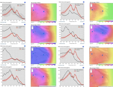
The second example of predictions (Fig. 4) refers to the forecast of PM2.5 in Shanghai on a relatively polluted day
(3 November 2017). All models predict the presence of rel-atively high concentrations over land (diurnal mean values of typically 100–150 µg m−3) with a steep negative gradient
towards the Chinese sea, where the concentrations are of the order of only 25–40 µg m−3. Observations made at different stations in this urban area show the occurrence of two succes-sive concentration peaks: one around 09:00–10:00 with con-centrations reaching about 180 µg m−3 and the second one at 15:00–16:00 with concentrations as high as 150 µg m−3. The ensemble mean forecast system predicts the occurrence of a single peak at about 07:00 with a PM2.5
concentra-tion of about 220 µg m−3. The forecast shows a gradual de-crease in the concentration during the afternoon that is in good agreement with the observation. The occurrence of the second peak in the afternoon, however, is missed by the en-semble prediction, even though a peak appears in some of the individual model calculations (WRF-Chem SMS, EMEP, and WRF–CMAQ) but often a few hours before it was
ac-tually detected by the monitoring stations. An inspection of the forecasts by the different models highlights the di-versity in the model results. IFS, CHIMERE, WRF-Chem-SMS, and EMEP overestimate the PM2.5concentrations
be-fore midday, while they provide values in good agreement with the observations in the afternoon and evening. WRF-Chem-MPIM underestimates the concentrations during the entire day. LOTOS-EUROS as well as WRF–CMAQ provide values that are in fair agreement with the observations in the morning but underestimate the concentrations in the after-noon.
A third example (Fig. 5) refers to the predicted concentra-tion of PM2.5on 25 October 2017 in Beijing. In this
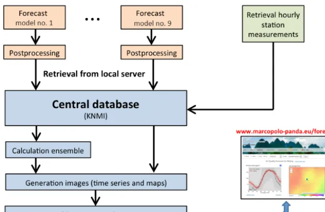
Figure 2.Structure of the operational multi-model forecast system with the nine model components. Postprocessed forecasts for the next 3 days provided by each model are sent to a central database maintained by the Royal Netherlands Meteorological Institute (KNMI). Ensem-ble medians and means are calculated and information (predicted daily variations in surface concentrations for 37 major Chinese cities, and maps of predicted diurnal mean surface concentrations) and are posted on http://www.marcopolo-panda.eu/forecast (last access: 7 Decem-ber 2018). Users in China are redirected to the mirror website maintained by SMS (http://116.62.195.108/, last access: 7 DecemDecem-ber 2018). The forecasts are compared with the median and mean observations provided by monitoring stations at different locations of the 37 cities.
exception of the WRF-Chem-MPIM model that shows mod-erate levels of pollution with an aerosol cloud localized in the urban area of Beijing. An examination of the results pro-vided by the individual models again shows large differences. Some models (CHIMERE, EMEP, LOTOS-EUROS, WRF-Chem-MPIM) calculate a slow and rather steady concen-tration increase during the day, while other models (WRF-Chem-SMS, WARMS-CMAQ-SMS, SILAM, and IFS) ex-hibit some irregular variations during the day. Most models overestimate the PM2.5 concentrations except for
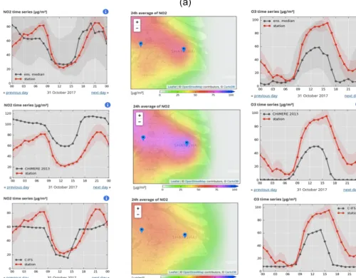
LOTOS-EUROS and WRF-Chem-MPIM, which predict concentra-tions with the same order of magnitude as the observaconcentra-tions at the monitoring stations. The last illustrative example refers to the forecast of nitrogen oxides and ozone in the Shanghai area on 31 October 2017 (Fig. 6a, b, and c). All models show that the NO2concentrations are highest in the boundary layer
of the urban areas, even though the calculated values may be different from model to model, and the dispersion of the species away from the urban centers may also be uneven. In all cases, predicted values above the ocean are very low, i.e., less than a few µg m−3. A band of high NO
2concentrations
extends from Shanghai in the northwest direction.
The median values of NO2in the city (Fig. 6a) are in good
agreement with the observed values, with nighttime concen-trations on the order of 60–80 µg m−3and substantially lower values during daytime resulting from the photolysis of the molecule by solar radiation. A minimum concentration of 25 µg m−3is reached around noon.
The diurnal variation in NO2 is well captured by most
models, in particular by CHIMERE (although the absolute values are too low), IFS, SMS, WRF-Chem-MPIM, and WARMS-CMAQ-SMS. The diurnal variation is somewhat underestimated in EMEP, LOTOS-EUROS, and WRF–CMAQ.
The ozone concentration (Fig. 6a–c) also exhibits a strong diurnal variation that, to a large extent, mirrors the NO2
variation. Measurements show a maximum value of nearly 100 µg m−3 reached at 15:00 and low nighttime concentra-tions (typically 10–30 µg m−3). The median concentrations, provided by the ensemble forecast system (Fig. 6a), are char-acterized by a similar diurnal variation but with lower am-plitude. The concentration reaches its maximum at 14:00, but the value of this maximum is only equal to 60 µg m−3. The values predicted for the night are generally somewhat smaller than the observation, with values of the order of 5– 10 µg m−3.
In the case of ozone, differences between model fore-casts are again substantial. The maximum concentra-tion values in the early afternoon are 50 µg m−3 for
CHIMERE, 62 µg m−3 for IFS, 85 µg m−3 for
Figure 3.Median concentrations of NO2(a), ozone(b), PM2.5(c), and PM10(d)predicted for the city of Xiamen on 13 October 2017
(black curve) and compared with the measured values (red curves). The dispersion of the forecasts by the individual models belonging to the ensemble is shown by the grey range, and the dispersion of the measured values at different stations in the city are depicted by the pink band.
5 Intercomparison of individual models
We now present an intercomparison of most of the models included in the operational MarcoPolo–Panda System. The participants to this intercomparison examined in detail the daily forecasts performed for the month of March 2017 with particular emphasis on the results obtained during the first 2 weeks of the month.
In the following sections, we present selected chemical fields derived by the different models that participated in the comparison exercise and highlight similarities and dif-ferences with the purpose of identifying the causes of the discrepancies between models and between models and ob-servations. We first examine monthly mean surface concen-trations obtained from a subset of the models involved in the intercomparison. We then compare the time evolution
asso-ciated with the model forecasts with observations made at specific surface measurement sites and present some corre-lations between calculated and measured concentrations at these sites.
5.1 Comparison of average fields
We first compare the March 2017 monthly mean concentra-tions of different chemical species calculated by seven mod-els (IFS, LOTOS-EUROS, EMEP, SILAM, WRF-Chem-MPIM, WRF-Chem-SMS, and CHIMERE) with surface measurements reported at different sites in the eastern part of China (http://pm25.in/).
Figure 4.Forecast by different models of PM2.5concentration during a polluted day in Shanghai on 3 November 2017. The graph in the top
panel of the first column represents the median concentration, and the individual forecasts provided by CHIMERE, IFS, WRF-Chem-SMS, WRF-Chem-MPIM, EMEP, LOTOS-EUROS, and WRF–CMAQ are shown by the other panels. Measured concentrations are represented by the red curves and model concentrations by the black curves.
forecasts, probably reflecting differences in the adopted emissions or in the atmospheric production resulting from the oxidation of volatile organic compounds in the plane-tary boundary layer. Observations indicate that CO concen-trations are generally higher than 900 ppbv, except near the southeastern coast and in the southwestern part of the coun-try, where the values are as low as 500 to 700 ppbv. The mod-els show considerably lower values, ranging from about 300 to 500 ppbv. The regions with the highest mean concentra-tions are located in the North China Plain (NCP), where ues higher than 1200 ppbv are recorded. Relatively high val-ues (close to 1000 ppbv) are also found in some urban areas (e.g., Hong Kong) near the south coast of the country.
The models provide a rather different picture: most of them substantially underestimate the CO concentrations, in particular WRF-Chem-SMS, WRF-Chem-MPIM, EMEP, and LOTOS EUROS. Higher concentrations are derived by
SILAM and IFS. These models, however, produce peak con-centrations in the region of the Sichuan Basin in contrast with the observations. Only IFS reproduces the high concentra-tions observed in northern China, probably because in this particular model the initial conditions are constrained by as-similated observations. Clearly, the performance of the mod-els regarding the calculation of CO concentrations is not sat-isfactory. The discrepancies may be attributed to an underes-timation of CO emissions, to errors in the lateral boundary conditions, or indirectly to an underestimation of the emis-sions for primary hydrocarbons.
In the case of NO2(Fig. 7b), the observations show that the
ar-Figure 5.Diversity of PM2.5forecasts in Beijing on 25 October 2017 by several models included in the ensemble of the MarcoPolo–Panda
prediction system. The ensemble median is shown by the top panels, and the individual forecasts provided by CHIMERE, IFS, WRF-Chem-MPIM, EMEP, WRF-Chem-SMS, SILAM, LOTOS-EUROS, and WARMS-CMAQ-SMS are shown by the other panels. Measurements are in red and model data in black.
eas but with values that are lower than those provided by the monitoring stations.
The mean surface ozone concentrations derived from mea-surements are lowest (about 20 ppbv) in the central part of China and highest (30–40 ppbv) near the east coast
(Shang-hai region), the south coast, and the western part of China. Since nitrogen oxides tend to titrate ozone, the models that predict high NO2concentrations derive the lowest ozone
val-ues (EMEP, SILAM, IFS). The high NO2concentrations
Figure 6.
used as shown in Fig. 1. CHIMERE, WRF-Chem-SMS, and to a lesser extent WRF-Chem-MPIM overestimate the mean ozone concentration during March. All models, however, produce a minimum in the ozone concentrations in northeast-ern China, a pattnortheast-ern that is not visible in the observational data (Fig. 7c).
Finally, in the case of PM2.5(Fig. 7d), the measurements
suggest the presence of high concentrations (higher than 80 µg m−3) in the region between Beijing and Shanghai. High abundances of PM2.5are derived in this region by IFS,
SILAM and to a lesser extent by LOTOS-EUROS, EMEP, CHIMERE, and WRF-Chem-SMS. Interestingly, most mod-els produce another marked hot spot in the region of the Sichuan Basin, while the observations suggest a less pro-nounced maximum with a more limited geographical extent.
5.2 Time evolution of median forecasts
We now focus on the time period during which the most in-tensive comparison between models has been performed. We first examine the time evolution of surface ozone, NO2, and
PM2.5produced by the different models for the time period
ranging from 1 to 15 March 2017 and for the three large metropolitan areas: Beijing, Shanghai, and Guangzhou. In Fig. 8, we compare the median concentrations of the three species with the median values derived from the different measurements provided by the network of instruments de-ployed in the three cities. The median model values are repre-sented by the red curves, while the shaded areas highlight the dispersion of the calculated concentrations around the me-dian values.
– Beijing. Here the predictions of the PM2.5
Figure 6.
one between 2 and 5 March and the second one on 11 March. In the case of NO2, the models reproduce
the daily variability reported by the monitoring stations fairly well, but on average, they slightly overestimate the concentrations values. The high concentrations ap-pearing between 2 and 5 March and between 10 and 11 March are well captured by the median of the mod-els. Finally, the models reproduce the diurnal variabil-ity in the ozone concentrations, but they underestimate these concentrations by typically 20 µg m−3.
– Shanghai. The calculated median concentrations of
PM2.5are in good agreement with the observations,
es-pecially between 10 and 15 March. During the first part of the simulation, the mean measured and calculated values are close, but the models produce peaks in the concentrations on 3, 6, 8, and 9 March that are higher than the observation. In the case of NO2, the
agree-ment between calculated and measured concentrations
is good. Again, the models severely underestimate the ozone concentrations.
– Guangzhou.The median concentration of PM2.5
pro-vided by the model is similar to the observation between 1 and 7 March. However, the model overestimates the concentrations between 7 and 11 March and underes-timates them between 12 and 14 March. For NO2, the
agreement between models and measurements is rela-tively good during the first days of the month, but the models overestimates the amplitude of the daily vari-ability observed after 6 March. Ozone is well simulated in this particular urban area, even though the daily peaks are sometimes over- or underestimated.
5.3 Statistical errors
calcu-Figure 6. (a)Diversity in the NO2and ozone forecasts made for Shanghai on 31 October 2017 as highlighted by the predictions from several
models included in the ensemble of the MarcoPolo–Panda system. The left and right columns show the diurnal variation in the predicted (black) and observed (red) NO2and ozone concentrations (µg m−3), respectively. The center column presents the geographical distribution
in the vicinity of Shanghai of the diurnal average predicted for the NO2concentration. The ensemble median is shown in the top row, and
two individual forecasts as provided by CHIMERE and IFS are shown in the middle and lower rows.(b)Same as in(a)but for the individual forecasts from WRF-Chem-SMS, WRF-Chem-MPIM, and EMEP.(c)Same as(a)but for the individual forecasts from LOTOS-EUROS, WRF–CMAQ, and WARMS-CMAQ.
lated statistical measures of the model results for the cho-sen period of 1–15 March 2017. These measures include the mean bias (BIAS), the mean normalized bias (MNMBIAS), the root mean square error (RMSE), the fractional gross error (FGE), and the correlation coefficient for ozone, NO2, and
PM2.5(Table 4). They apply to the data for the 37 cities
con-sidered in the MarcoPolo–Panda forecast system. The same statistical measures are also provided for the ensemble me-dian.
When examining the mean bias of the ensemble me-dian, the values are equal to−14.7,−3.0, and+3.7 µg m−3 for ozone, NO2, and PM2.5, respectively, to be compared
to mean concentration values of the order of 50 µg m−3
for these three different species. Table 4 shows that in the case of ozone, individual models are characterized by bi-ases ranging from−25.8 (SILAM) to+13.2 µg m−3 (WRF-Chem-SMS), with the smallest absolute value equal to 5.9 µg m−3(CHIMERE) The corresponding numbers range
from −20.7 µg m−3 (LOTOS-EUROS) to +11.2 µg m−3 (EMEP) with the smallest absolute bias of −2.0 µg m−3 (IFS) for NO2. For PM2.5, they range from −4.7 µg m−3
(LOTOS-EUROS) to +39.6 µg m−3 (IFS) with the small-est absolute value equal to −2.0 µg m−3 (CHIMERE). In general, during the period chosen for the intercomparison, the models underestimate the ozone and NO2
Figure 7.Monthly mean surface concentrations of(a)CO,(b)NO2,(c)ozone (ppbv), and(d)PM2.5(µg m−3) provided for the month of
Table 4.For the period 1 to 15 March 2017, statistical measures (mean bias (BIAS), mean normalized bias (MNMBIAS), root mean square error (RMSE), FGE (fractional gross error), and correlation coefficients) calculated for the forecast of O3, NO2, and PM2.5concentrations
for all models and for the ensemble median at all stations/cities, for which the MarcoPolo–Panda Forecast is available. The correlation is based on 1-hourly data.
Ensemble CHIMERE IFS WRF-Chem SILAM WRF-Chem EMEP LOTOS-EUROS
Median SMS MPIM
BIAS (µg m−3) O3 −14.7 −5.9 −13.1 13.2 −25.8 −23.9 −23.3 −4.0
NO2 −3.0 −4.8 −2.0 −4.2 −3.1 8.4 11.2 −20.7
PM2.5 3.7 −2.0 39.7 −4.5 21.7 5.5 12.4 −4.7
MNMBIAS (%) O3 −41 % −24 % −51 % 13 % −74 % −69 % −74 % −7 %
NO2 −8 % −18 % −13 % −19 % −11 % 13 % 15 % −52 %
PM2.5 8 % −4 % 44 % −18 % 22 % 11 % 9 % −7 %
RMSE (µg m−3) O3 32.8 27.0 29.4 41.8 44.6 44.7 42.9 37.2
NO2 21.8 24.4 23.1 31.9 28.5 28.9 34.0 34.4
PM2.5 30.2 31.5 71.3 35.8 47.7 39.1 52.4 27.3
FGE (%) O3 70 % 58 % 72 % 64 % 99 % 97 % 99 % 65 %
NO2 38 % 45 % 44 % 53 % 51 % 43 % 48 % 66 %
PM2.5 38 % 44 % 62 % 54 % 52 % 49 % 47 % 39 %
Corr. coeff. O3 0.60 0.70 0.72 0.45 0.32 0.32 0.39 0.38
NO2 0.64 0.62 0.65 0.47 0.41 0.50 0.46 0.31
PM2.5 0.62 0.55 0.47 0.54 0.66 0.36 0.49 0.64
Table 5.Best model performance.
Statistical variable Best performance ozone Best performance NO2 Best performance PM2.5
Mean bias LOTOS-EUROS IFS CHIMERE
RMSE CHIMERE IFS LOTOS-EUROS
Correlation coefficient IFS WRF-Chem MPIM SILAM
ble also shows that the RMSE for the median values for ozone, NO2, and PM2.5are 32.8, 21.8, and 30.2 µg m−3,
re-spectively. With some exceptions (CHIMERE and IFS for ozone, LOTOS-EUROS, for PM2.5), these values are lower
than the RMSE derived by individual models. The highest values for RMSE are 44.7 µg m−3 (WRF-Chem-MPIM) in the case of ozone, 34.4 (LOTOS EUROS) in the case of NO2,
and 71.3 (IFS) in the case of PM2.5. The smallest RMSE
are equal to 27.0 µg m−3(CHIMERE) in the case of ozone, 23.1 µg m−3 (IFS) in the case of NO2, and 27.3 µg m−3 in
the case of PM2.5(LOTOS-EUROS). The correlation
coeffi-cient for the ensemble median is of the order of 0.6 for the three species, which in most cases is higher than the values derived from individual model forecasts. There are a few ex-ceptions, however. The correlation coefficients are higher in the forecast of ozone by CHIMERE (0.70) and IFS (0.72), in the case of NO2 by IFS (0.65), and in the case of PM2.5
by SILAM (0.66) and LOTOS-EUROS (0.64). Table 5 sum-marizes the models that have achieved the best performance from the point of view of the mean bias, the RMSE, and the correlation coefficient.
5.4 Time evolution of individual forecasts
The time evolution of predicted concentration values at Bei-jing by five different models involved in the intercomparison is provided in Fig. 9 for the period of 1–15 March 2017. An examination of the figure shows that, during most days, the daytime height of the PBL reaches 2500–3000 m with an ex-ception on 2 to 5 March, when the height does not exceed 1000 m. Interestingly, during this period, the observed con-centration of particulates, of NO2, and of SO2, strongly
Figure 9.Forecast of the chemical concentrations of ozone, NO2, PM2.5, and PM10at Beijing between 1 and 15 March 2017 by the different models involved in the intercomparison conducted in the present study. The calculated values of Ox=O3+NO2as well as the height of
the planetary boundary layer (PBL) are also shown. The mean values from the measurements made at the different monitoring stations of Beijing are shown by the thick red line.
calculation of the PBL height makes use of meteorological data provided by the IFS model.
In most cases, the models capture the day-to-day variabil-ity in the species concentrations relatively well. The agree-ment with observations is generally good in the case of PM2.5
and PM10, except in the case of the IFS model, which
consid-erably overestimates the concentrations, mainly because of a regional overestimation of the OM emissions and a lack of a diurnal variation in the emission. The anthropogenic OM emissions in IFS are parameterized based on anthropogenic CO emissions following Spracklen et al. (2011). The rela-tively high CO emission in this region may require a re-duced conversion factor between OM and CO emissions. The main contribution to PM overestimation of IFS came from the nighttime values (see next section). Since nighttime over-estimation also occurs for NO2, a lack of vertical mixing
during the night in IFS could cause the nighttime overesti-mation of the surface values. As already noted, the models tend to underestimate the ozone concentrations, perhaps due to a slight overestimation of the nitrogen oxide concentra-tions. Another possible explanation is an underestimation of the VOC sources. Routine measurements of VOCs, however, are not available. The need for such measurements, however, needs to be stressed.
The model comparison reported here also shows differ-ences between models in the case of NO, which should prob-ably be attributed to differences in the emissions and emis-sion injection heights of this species and in the formulation of vertical mixing in the boundary layer. Here again, measure-ments of NO in addition to those of NO2and ozone would
be useful. Finally, one notes in Fig. 9 the relatively good agreement between models (with the exception of the IFS and the WRF-Chem-SMS model) regarding the time evolu-tion of odd oxygen (Ox=O3+NO2). The models, however,
slightly underestimate the absolute values of the Ox
concen-tration.
5.5 Diurnal variations
In order to evaluate the behavior of the different models re-garding their ability to reproduce the diurnal variation in the surface concentrations of ozone, NO2, and PM2.5, we have
calculated the mean diurnal variations over the period of 1– 15 March 2017 averaged for the 34 cities included in our analysis (3 of the 37 cities, located in the western part of the country and adopted in the MarcoPolo–Panda prediction system have not been considered in this analysis). The re-sulting results are shown in Fig. 10 for ozone and NO2
diur-Figure 10.Upper row: diurnal variation in ozone (left), NO2(middle), and Ox=NO2 +O3(right) for the period 1–15 March 2017 for
all cities included in the MarcoPolo–Panda Prediction system for all seven models and the ensemble median and the observations (red line). Middle row: root mean square error (RMSE) for ozone (left), NO2(middle), and Ox(right). Lower row: bias for ozone (left), NO2(middle),
and Ox(right) for all models and for the ensemble median (black line).
nal evolution of Ox (expressed in ppbv) defined as the sum
of the ozone and NO2mixing ratios. This last chemical
vari-able has the advantage that it is not affected by the fast inter-change (null cycle) between ozone and NO2by the reactions
NO+O3, NO2 +hv, and O +O2 +M. Since this cycle
tends to transfer “odd oxygen” from ozone to NO2after
sun-set and from NO2to ozone after sunrise, the Oxvariable is
less variable than its two components NO2and O3over a
di-urnal cycle. Figure 10 shows that, when averaging over the 34 largest Chinese cities, the diurnal variation in the ensemble median is in good agreement with the observation in the case of NO2. In the case of ozone, the median values are
some-what underestimated in late morning and in the afternoon. A similar situation is found in the case of Ox. The RMSE for
ozone and NO2, also shown on the figure, is generally lower
in the case of the ensemble median than for the individual models. In the case of PM2.5, however, the RMSE of the two
models CHIMERE and IFS are smaller than the RMSE of the ensemble median (not shown here). The mean bias of the en-semble median for NO2and ozone is generally smaller than
that of the individual models. In the case of Ox, some models
exhibit a positive bias (WRF-Chem SMS), while others (e.g., SILAM) are characterized by a negative bias.
Figure 11a, b, and c show similar estimates of the diurnal variation in the three large cities of China: Beijing, Shang-hai, and Guangzhou. These graphs show that the ozone fore-cast from the ensemble median is lower than observed val-ues during the entire day both in Beijing and in Shanghai. In Guangzhou, however, ozone is slightly overestimated by the prediction. In the case of NO2, the surface concentrations are
overestimated in Beijing and to a lesser extent in Shanghai, with the largest overprediction occurring during nighttime, when the planetary boundary layer is very thin and vertical mixing almost shut off. At the same time, ozone is negatively biased due to its efficient titration by NOx. In the three cities,
the RMSE of NO2, ozone, and Oxappear to be largest at
sun-set. Thus, a general issue with the MarcoPolo–Panda predic-tion system is the overestimapredic-tion of surface NO2and the
un-derestimation of ozone concentrations during the nighttime. In the case of PM2.5, one of the models involved (IFS)
Figure 11.
This issue may again reflect a problem with the formulation of species dispersion in the planetary boundary layer. It may also be due to the lack of specified diurnal variation in the emission of primary pollutants as well as to the increased nighttime stability.
6 Approaches to improve the forecasts
The intercomparison presented in the previous sections pro-vides useful information and represents the basis on which the accuracy of the model predictions can be improved. Since the models have been developed fairly independently and the choices about input parameters such as emissions, chemical schemes, and adopted weather forecasts have been based on best judgement by these individual teams, a statistical treat-ment of the model results (e.g., determination of averages and standard deviation) provides, in general, more reliable information than the data provided by the individual model components of the ensemble. The examination of the model output reveals, however, some systematic biases that could be reduced by identifying the likely cause of these errors.
A simple approach is to recognize that the failure of mod-els to correctly predict air quality could result from several factors: (1) errors in the adopted emissions and the formu-lation of boundary layer dispersion best diagnosed by an-alyzing the ability of the model to reproduce the monthly mean surface concentrations of chemical species; (2) errors or omission in the adopted chemical scheme leading to in-accuracies in the calculated mean diurnal variations in the concentrations of secondary species; and (3) inaccuracies in the adopted weather forecasts leading to poorly calculated day-to-day variations in the calculated chemical fields. In this later case, one should distinguish between fundamental model biases (i.e., the representation of PBL mixing, a bias that is intrinsic to the models) and the increasing error in the forecast of synoptic weather patterns as the model integration proceeds. This probably provides an oversimplified view of the causes of errors in chemical weather forecasts, but it of-fers a simple approach to address some issues in the models and hence to improve the predictions.
Figure 11.
same meteorological forecasts. Remaining differences be-tween the models will be due in large part (although not ex-clusively) to the adopted chemical scheme and the formula-tion of boundary layer processes. An addiformula-tional step would be to bring the different formulations of chemistry closer to-gether by at least harmonizing the adopted rate constants and using the same module to calculate photodissociation rates. Finally, it would be interesting to assess the differences in chemical weather predictions resulting from the adopted me-teorological forecasts. In particular, it would be important to better constrain the differences in the photolysis rates result-ing from the adopted or calculated concentrations of aerosols and in cloudiness. One single model could be run for several days with the weather predictions produced by different me-teorological centers.
Finally, a few specific issues from the present intercom-parison require attention:
1. Most models overestimate the surface levels of NO2and
PM2.5 as well as other species emitted at the surface,
specifically during nighttime. The largest discrepancies appear around 18:00 LT when the surface cools and the boundary layer collapses and the emitted species remain
trapped in the lowest model layers. Evidently, these models underestimate the vertical exchanges between layers probably produced by the turbulence thermally or mechanically generated by the presence of buildings. Such effects are not accounted for in models that do include a specialized urban formulation. The overesti-mation of NO2 during nighttime leads to the titration
Figure 11. (a)Same as Fig. 10 but for the urban area of Beijing. The statistical variables for PM2.5are also included.(b)Same as Fig. 10 but for the urban area of Shanghai. The statistical variables for PM2.5are also included.(c)Same as Fig. 10 but for the urban area of Guangzhou.
The statistical variables for PM2.5are also included.
Figure 12.Annually averaged diurnal evolution of the PM2.5
con-centrations in the city of Chengdu simulated for different values of the particulate injection height. Calculations by the LOTOS-EUROS (LE) model.
shows diurnal cycles of the simulated PM2.5
concentra-tions in the city of Chengdu, averaged over an entire year. The updated emission heights clearly have a large (positive) impact on the simulations.
2. Daytime concentrations of ozone are generally under-estimated in most regions of eastern China, even when the level of NO2 is in reasonable agreement with the
values reported by the monitoring stations. The discrep-ancy could be caused by an underestimation of the emis-sions of some VOCs, especially in urban areas where ozone is often VOC-limited. More work is required to investigate this question.