https://doi.org/10.5194/gmd-11-1591-2018 © Author(s) 2018. This work is distributed under the Creative Commons Attribution 4.0 License.
Continuous state-space representation of a bucket-type
rainfall-runoff model: a case study with the GR4 model
using state-space GR4 (version 1.0)
Léonard Santos, Guillaume Thirel, and Charles Perrin
Irstea, UR HYCAR, 1 rue Pierre-Gilles de Gennes, 92160 Antony, France Correspondence:Léonard Santos ([email protected])
Received: 23 October 2017 – Discussion started: 5 December 2017
Revised: 16 February 2018 – Accepted: 22 March 2018 – Published: 19 April 2018
Abstract. In many conceptual rainfall–runoff models, the water balance differential equations are not explicitly formu-lated. These differential equations are solved sequentially by splitting the equations into terms that can be solved analyti-cally with a technique called “operator splitting”. As a result, only the solutions of the split equations are used to present the different models. This article provides a methodology to make the governing water balance equations of a bucket-type rainfall–runoff model explicit and to solve them continu-ously. This is done by setting up a comprehensive state-space representation of the model. By representing it in this way, the operator splitting, which makes the structural analysis of the model more complex, could be removed. In this state-space representation, the lag functions (unit hydrographs), which are frequent in rainfall–runoff models and make the resolution of the representation difficult, are first replaced by a so-called “Nash cascade” and then solved with a robust numerical integration technique. To illustrate this method-ology, the GR4J model is taken as an example. The substi-tution of the unit hydrographs with a Nash cascade, even if it modifies the model behaviour when solved using opera-tor splitting, does not modify it when the state-space repre-sentation is solved using an implicit integration technique. Indeed, the flow time series simulated by the new represen-tation of the model are very similar to those simulated by the classic model. The use of a robust numerical technique that approximates a continuous-time model also improves the lag parameter consistency across time steps and provides a more time-consistent model with time-independent parameters.
1 Introduction
1.1 On the need for an adequate mathematical and computational hydrological model
Hydrological modelling is a widely used tool to manage rivers at the catchment scale. It is used to predict floods and droughts as well as groundwater recharge and water qual-ity. In a review on the different existing hydrological models, Gupta et al. (2012) determined that all the existing models follow three modelling steps:
– establish a conceptual representation of reality,
– represent this conceptualization in a mathematical model,
In the context of this study, bucket-type models are ad-vantageous because, even if the concepts are often well doc-umented, this is not the case of the mathematical and the computational models. In the models’ documentations, the water balance equations that would govern the models are rarely explicitly formulated (Clark and Kavetski, 2010). The authors of the models often specify the discrete time equa-tions, i.e. the result of the analytical or numerical temporal integration of the governing water balance equations. The problem is that the temporal resolution of the differential governing equations is part of the computational model. As a consequence, when the discrete time equations are the only ones available, the real mathematical model does not appear clearly. In addition, the descriptions of the numerical method used to solve the water balance equations and to obtain these discrete equations are rarely detailed.
However, several studies in the last decade (see for ex-ample Clark and Kavetski, 2010; Kavetski and Clark, 2010; Schoups et al., 2010) point out that the numerical solutions implemented to solve the differential equations that govern the models are sometimes poorly adapted. Clark and Kavet-ski (2010) showed that the use of the explicit Euler scheme (which is frequent for this type of model) can introduce sig-nificant errors in the simulated variables compared to more stable numerical schemes. Moreover, other studies prove that poorly adapted numerical treatment causes discontinuities and local optima in the parameter hyperspace (Kavetski et al., 2003; Kavetski and Kuczera, 2007; Schoups et al., 2010). This results in problems efficiently calibrating the models and in uncertainty on parameter values.
Another numerical approximation is commonly applied for bucket-type models: the operator splitting (OS) technique (Kavetski et al., 2003). The aim is to split a differential equation into more simple equations that can be solved an-alytically in order to reduce inaccuracies in the numerical treatment. In the case of hydrological modelling, operator splitting results from the sequential calculation of processes such as runoff, evaporation and percolation (Schoups et al., 2010). Kavetski et al. (2003), Clark and Kavetski (2010) and Schoups et al. (2010) identified several widely used models in which the differential equations are solved using this type of treatment, e.g. VIC (Wood et al., 1992), Sacramento (Bur-nash, 1995) and GR4J (Perrin et al., 2003). However, even if OS may reduce numerical errors, Fenicia et al. (2011) cite several limitations to its use in hydrology. Indeed, it is phys-ically unsatisfying to separate the different processes in time because, in reality, they are concomitant. In addition, it cre-ates numerical splitting errors that are difficult to identify.
According to different studies, an inadequate numerical treatment like OS can lead to inconsistencies in flux simula-tions (see for example the study conducted by Michel et al., 2003, on an exponential store). It may also create incon-sistencies in the model state variables (Clark and Kavetski, 2010; Kavetski and Clark, 2010). This results in the model inaccurately simulating flows.
For these reasons, it is important to use a robust numer-ical treatment to better estimate the other uncertainties (for example, parameter uncertainty).
1.2 Scope of this study
The first step to improve the numerical treatment of rainfall– runoff models is to properly separate the mathematical model from the computational model (Kavetski and Clark, 2010; Gupta et al., 2012). This article proposes a method to do this by setting up a continuous state-space representation of a rainfall–runoff model. A state-space representation is a ma-tricial function of a system that depends on input, output and state variables. At all times, the system is described by the values of its state variables (referred to as “states” in this ar-ticle). In the case of rainfall–runoff models, inputs can be potential evapotranspiration and precipitation and output can be the flow at the outlet of the catchment. The soil water con-tent or the amount of water in the hydrographic network are physical examples of possible state variables. The level of the bucket-type model stores is a conceptual example of pos-sible state variables. This state-space representation will give the governing equations to be solved over time. This resolu-tion will be proceeded by using an OS technique to be used as a comparison point and by using a more robust numer-ical technique, i.e. implicit Euler with an adaptive sub-step number. The model solved by implicit Euler will be called continuous state-space because it approximates a continuous model. By opposition, the OS state-space representation will be named as discrete.
In addition to a clearer mathematical model, we hope that the state-space representation will gain stability due to the direct implementation of the time step in the numerical reso-lution. We thus hope to obtain more stable parameter values across time steps (Young and Garnier, 2006).
To illustrate the methodology proposed, the widely used GR4J model (Perrin et al., 2003) will be taken as an ex-ample. Indeed, this model is currently implemented using the OS technique. A state-space representation will be set up, following the GR4J’s conceptualization of the hydrolog-ical processes as much as possible. Its behaviour, both with a discrete and a continuous solving, will be compared to the current formulation of the GR4J model on a wide range of French catchments with different time steps (day and hour), in terms of performance and parameters.
2 GR4 and its new state-space representation
intro-E P
S
Q x1
R F(x2)
x3
Q9
Qr
Quh
Perc
Pn
Pn-Ps
Pr
Ps
En
Es
Q1
F(x2)
Qd
E P
S
Q x1
R F(x2)
x3
Q9
Qr
UH2
Quh
2x4
Perc
Pn
Pn-Ps
Pr
Ps
En
Es
Q1
F(x2)
Qd
(a)
(b)
...
Nash cascade
Sh,1
Sh,2
Sh,nres
QSh,1
QSh,2
QSh,nres-1
Production store Interception
Routing store Unit hydrograph
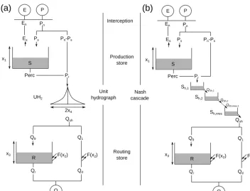
Figure 1.Schemes of the reference GR4 model (a, Perrin et al., 2003) and the state-space(b)structures.P: rainfall;E: potential evapotran-spiration;Q: streamflow;xi: model parameter; other letters are model state variables or fluxes. A Nash cascade replaces the unit hydrograph
in the state-space representation.
duced in the GR4 state-space form is given in Sect. 2.3. The continuous differential equations of the state-space form are described in Sect. 2.4. The adaptations needed to change the model time step will be described in Sect. 2.5.
2.1 Reference GR4 model
GR4 (Perrin et al., 2003) is a lumped bucket-type daily rainfall–runoff model with four free parameters. It is widely used for various hydrological applications in France (Grouil-let et al., 2016; van Esse et al., 2013) and in other countries (Dakhlaoui et al., 2017; Seiller et al., 2017). It has shown good performances on a wide range of catch-ments (Coron et al., 2012). The equations of the reference GR4J model (Perrin et al., 2003) are the result of the inte-gration of the water balance equations at a discrete time step (here the daily or hourly time step).
The version of GR4 used here is slightly different from the one presented by Perrin et al. (2003) because the two unit hydrographs were replaced by a single one placed before the flow separation (Fig. 1a, Mathevet, 2005). This simplifica-tion of the model does not substantially change the resulting simulated flows.
The equations of the model are given by Perrin et al. (2003) and listed in Table 1. GR4 represents the rainfall– runoff relationship at the catchment scale using an intercep-tion funcintercep-tion, two stores, a unit hydrograph and an exchange
function (see Fig. 1a). The model structure can be split into water balance and routing operators.
The water balance operators evaluate effective rainfall (i.e. the part of rainfall that will reach the catchment outlet) by estimating several quantities: actual evaporation, storage within the catchment and groundwater exchange. It involves an interception function and a production (soil moisture ac-counting) store (Sin Fig. 1a). The interception corresponds to a neutralization of rainfall by potential evapotranspiration. The remaining rainfall (Pn), if any, is split into a part going
into the production store (Psin Fig. 1a) and a complementary
part (Pn−Ps in Fig. 1a) that is directed to the routing
com-ponent of the model. The quantity of rainfall that feeds the production store depends on the level of water in the store at the beginning of the time step. In case there is remaining en-ergy for evapotranspiration after interception (Enin Fig. 1a),
some water is evaporated from the production store at an ac-tual rate depending on the level of the production store (Esin
Fig. 1a). The higher the level is at the beginning of the time step, the closerEsis toEn. Thus, the production store
repre-sents the evolution of the catchment moisture content at each time step. The last water balance operator is a groundwater exchange term (F in Fig. 1a, positive or negative), which acts on the routing part of the model.
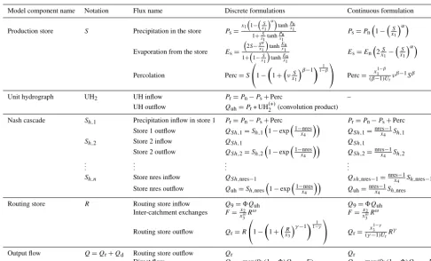
per-Table 1.Details of the equations of the GR4 model and discrete and continuous formulations. The discrete formulations are the continuous equations integrated individually over the modelling time step using the operator splitting technique while continuous equations correspond to the terms of the water balance differential equation of each store. * The values of UH2are calculated using Eq. (17) in Perrin et al. (2003). Please note that the two discrete formulations use either the unit hydrograph equations or the Nash cascade formulation.
Model component name Notation Flux name Discrete formulations Continuous formulation
Production store S Precipitation in the store Ps=
x1
1−
S x1
α
tanhPn
x1 1+S
x1tanh
Pn
x1
Ps=Pn
1−
S
x1
α
Evaporation from the store Es=
2S−Sα x1
tanhEn
x1 1+
1−S x1
tanhEn
x1
Es=En
2xS
1−
S
x1
α
Percolation Perc=S
1−
1+
νxS
1
β−1
1
1−β
Perc=
x11−β
(β−1)Utν
β−1Sβ
Unit hydrograph UH2 UH inflow Pr=Pn−Ps+Perc –
UH outflow Quh=Pr∗UH(2∗)(convolution product)
Nash cascade Sh,1 Precipitation inflow in store 1 Pr=Pn−Ps+Perc Pr=Pn−Ps+Perc
Store 1 outflow QSh,1=Sh,1
1−exp
1−nres
x4
QSh,1=nresx4−1Sh,1
Sh,2 Store 2 inflow QSh,1 QSh,1
Store 2 outflow QSh,2=Sh,2
1−exp1−xnres
4
QSh,2=nresx4−1Sh,2
. .
. ... ... ...
Sh,n Store nres inflow QSh,nres−1 Qsh,nres−1=nresx4−1Sh,nres−1
Store nres outflow Quh=Sh,nres
1−exp
1−nres
x4
Quh=nresx4−1Sh,nres
Routing store R Routing store inflow Q9=8Quh Q9=8Quh
Inter-catchment exchanges F=x2
xω
3
Rω F=x2
xω
3 Rω
Routing store outflow Qr=R
1−
1+
R
x3
γ−11−γ1
Qr=
x13−γ
(γ−1)UtR
γ
Output flow Q=Qr+Qd Routing store outflow Qr Qr
Direct flow Qd=max(0;(1−8)Quh−F ) Qd=max(0;(1−8)Quh−F )
colation term (Perc in Fig. 1a) from the production store, which generally represents a small amount of water. The to-tal amount (Prin Fig. 1a) is lagged by a symmetric unit
hy-drograph and then split into two flow components. The main component (90 % ofPr,Q9in Fig. 1a) is routed by a
nonlin-ear routing store (Rin Fig. 1a). The complementary compo-nent (10 % ofPr,Q1in Fig. 1a) directly reaches the outlet.
The groundwater exchange term (F) is added or removed from the routing store and from theQ1component.
The simulated flow at the catchment outlet (Qin Fig. 1a) is the sum of the outputs of the two flow components (Qrand
Qdin Fig. 1a).
Four free parameters (calledx1,x2,x3andx4) are used to
adapt the model to the variety of catchments. Their meanings are given in Table 2.
As mentioned in the introduction, the governing water bal-ance equations of the model are solved using OS. By con-sidering that inputs to the store are added at the beginning of the time step as Dirac functions (Michel, 1991), it be-comes possible to find analytical expressions of the model processes when equations are integrated over the time step. Consequently, the model processes are treated sequentially.
2.2 A state-space formulation for the GR4 model
To create this state-space representation, it is important to identify the different model state variables. In the GR4 model, two obvious states are the levels of the production and routing stores. The main challenge to describe the state-space formulation is to deal with the unit hydrograph. The discrete form used in GR4 corresponds to a convolution product in the state space as implemented in SUPERFLEX (Kavetski and Fenicia, 2011). This convolution product makes the mathe-matical resolution of the model that is necessary for the con-tinuous version that will be introduced in Sect. 2.4 more com-plex. Here we chose to replace this unit hydrograph with a se-ries of linear stores in order to simplify this resolution. The use of stores is also convenient because it creates a model that is only composed of stores.
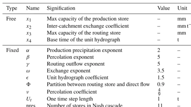
Table 2.Meaning of the free and fixed parameters (from Perrin et al., 2003, except forUtand nres).
Type Name Signification Value Unit
Free x1 Max capacity of the production store – mm
x2 Inter-catchment exchange coefficient – mm t−1
x3 Max capacity of the routing store – mm
x4 Base time of the unit hydrograph – t
Fixed α Production precipitation exponent 2 –
β Percolation exponent 5 –
γ Routing outflow exponent 5 –
ω Exchange exponent 3.5 –
Unit hydrograph coefficient 1.5 –
8 Partition between routing store and direct flow 0.9 –
ν Percolation coefficient 49 –
Ut One time step length 1 t
nres Number of stores in Nash cascade 11 –
decided to fix the number of stores and to only consider the outflow coefficient as a free parameter. This choice will be discussed in the following section (Sect. 2.3). With this type of model, the outflow of the last store has a similar shape to a unit hydrograph.
2.3 Parameterization of the Nash cascade
As introduced in the previous section, the Nash cascade has two parameters, namely the number of stores and the out-flow coefficient. The number of stores can only take integer values, which is an issue for automatic calibration because it introduces threshold effects. As a consequence, the number of stores was not optimized automatically and the outflow coefficient is the preferential parameter to calibrate.
To obtain a response that is equivalent to the GR4 unit hy-drograph response, we attempted to determine whether a re-lationship exists between the Nash cascade parameters and the GR4x4parameter. To manage this, the determination of
the Nash cascade parameter is based on the comparison of the impulse response of the Nash cascade and the response of the unit hydrograph.
The impulse response of the Nash cascade is (Nash, 1957)
hNash(t )=
k 0(nres)(kt )
nres−1exp(−kt ), (1)
wherehNash(t )is the impulse response of the Nash cascade
at timet, nres is the number of stores,kis the outflow coef-ficient (t−1) and0(nres)corresponds to the gamma function
of nres.
The impulse response of the GR4 symmetrical unit hydro-graph is (Perrin et al., 2003)
hUH(t )=
2.5 2x4
t
x4
1.5
, for 0≤t≤x4
2.5 2x4
2− t
x4
1.5
, forx4< t≤2x4
0 , fort >2x4
, (2)
wherehUH(t )is the impulse response of the unit hydrograph
at timetandx4is the time to peak of the hydrograph.
The Nash cascade parameters are calculated depending on x4 in such a way that the time to peak and the peak flow
would be the same for the two impulse responses. Accord-ing to Szöllösi-Nagy (1982), the time to peak of the Nash cascade is equal to
tp=
nres−1
k (3)
and the peak flow is equal to qp=
k
0(nres)(nres−1)
nres−1exp(1−nres). (4)
Using Eq. (2), the time to peak of the GR4 unit hydrograph is equal to
tp=x4 (5)
and the peak flow to qp=
1.25 x4
. (6)
So, from these values the following system can be deduced:
x4=
nres−1 k 1.25
x4
= k
0(nres)(nres−1)
nres−1exp(1−nres)
0 1 2 3 4 5 6
0.0
0.2
0.4
0.6
0.8
1.0
Time (t)
Outflo
w q(t)
Unit hydrograph response with x4 = 2
Nash cascade response with x4 = 2
Figure 2.Impulse response withx4=2 time steps for the unit hy-drograph of GR4 (dotted line) and the Nash cascade with nres=11 stores andk=11−1
x4 (dashed line).
which can be transformed into
k=nres−1
x4
1.25=(nres−1)
nres
0(nres) exp(1−nres)
. (8)
A nres=11 is the best integer approximation to solve the second equation of Eq. (8). The outflow coefficient is de-duced from this number of stores and fromx4. By fixing the
parameters in this way, only thex4parameter has to be
cali-brated. This method allows a direct comparison between the parameters of the Nash cascade and the parameter of the unit hydrograph. For a given x4 parameter, the unit hydrograph
and the Nash cascade impulse responses have the same time to peak and the same peak flow (see the dotted and the dashed curve in Fig. 2).
Using this formula, the x4 parameters of the two
mod-els are equivalent and it can be argued that their meaning is nearly identical.
Fixing the number of stores in the Nash cascade also pro-vides another advantage. Indeed, one of the potential issues that arises when replacing the unit hydrograph with a Nash cascade was the equifinality with the routing store. Given that the recession curve of the cascade is theoretically infinite, it could have the same function as the routing store. Calculat-ing the parameters of the cascade regardCalculat-ing thex4parameter
makes it possible to reduce the possibility of an infinite im-pulse response.
2.4 Continuous differential equations of the state-space model
Once the model is only represented by stores, a differential equation can be written for each store (details are provided in Table 1). For the production and routing stores, the equations
were built by adding all the processes that affect the stores. For example, the differential equation for the production store is the sum of the differential equations of evaporation, rainfall and the percolation (respectively,Es,Psand Perc in
Fig. 1). This means that all the processes that are a function of this state are treated simultaneously, unlike the initial model version in which the processes are treated sequentially. The state-space representation of the Nash cascade is the same as the one proposed by Szöllösi-Nagy (1982).
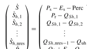
The resulting model is composed of the differential equa-tions governing the states’ evolution (here represented as a vector in the Eq. (9), taking into account nres stores in the Nash cascade):
˙
S
˙
Sh,1
˙
Sh,2
.. .
˙
Sh,nres
˙
R
=
Ps−Es−Perc
Pr−QSh,1
QSh,1−QSh,2
.. . QSh,nres−1−Quh
Q9+F−Qr
. (9)
The notationS˙stands for ddSt, the derivative ofSagainst time t and the different elements of this equation are specified in Table 1.
The output equation to calculate the instantaneous output flow (q(t )in Eq. 10) completes the model:
q(t )=Qr+Qd. (10)
The different elements in Eqs. (9) and (10) are shown in Ta-ble 1.
The input, state variable and output values are as follows.
– Inputs.EnandPnare the potential evapotranspiration
(after the interception) and the precipitation amounts after the interception phase (mm t−1). We decided to keep the interception out of the state-space representa-tion because it is not represented by a store in the refer-ence GR4J and we wanted to avoid introducing an ad-ditional difference between the state-space and the ref-erence models.
– Output.Qis the output flow; it corresponds to the
inte-gration ofq(t )(Eq. 10) over the time step.
– State variables.S,RandSh,kare respectively the levels
of the production store, the routing store and the Nash cascade store numberk (withk∈ {1,· · ·,nres}) in mil-limetres.
– Fluxes.Ps andEs are, respectively, the rainfall added
to the production store and the evapotranspiration ex-tracted from the production store. Perc is the outflow from the production store. Pr is the amount of
wa-ter that reaches the model routing operators. QSh,k is
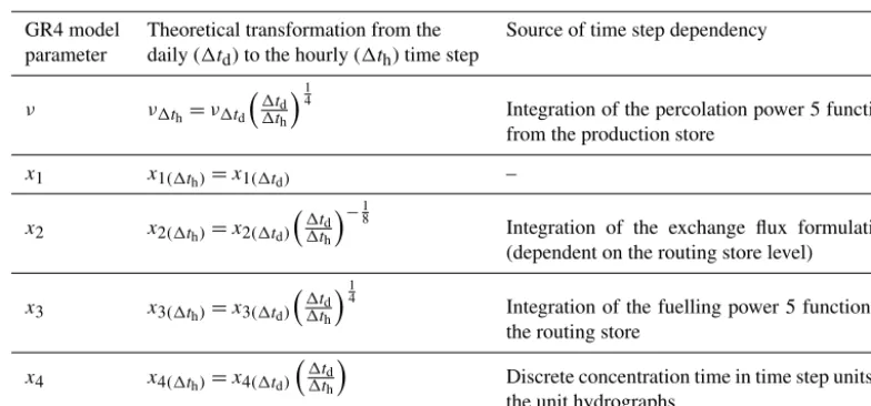
Table 3.Temporal transformations of the GR4 parameters (Ficchí et al., 2016).
GR4 model Theoretical transformation from the Source of time step dependency parameter daily (1td) to the hourly (1th) time step
ν ν1th=ν1td
1td
1th
14
Integration of the percolation power 5 function from the production store
x1 x1(1th)=x1(1td) –
x2 x2(1th)=x2(1td)
1t
d
1th
−18
Integration of the exchange flux formulation (dependent on the routing store level)
x3 x3(1th)=x3(1td)
1td
1th
14
Integration of the fuelling power 5 function of the routing store
x4 x4(1th)=x4(1td)
1t
d
1th
Discrete concentration time in time step units of the unit hydrographs
k∈ {1,· · ·,nres−1}).Quhis the outflow of the Nash
cas-cade store number nres (this notation is used to be con-sistent with the discrete model).Q9andQrare,
respec-tively, the inflow and the outflow of the routing store and F is the inter-catchment groundwater exchange.Qdis
the outflow of the complementary flow component. The parameter meanings are explained in Table 2. The model is constructed to ensure that the parameters (x1,· · ·, x4in the
equations) have the same meaning in the continuous model and in the discrete GR4. The state-space formulation was sought to be as close as possible to the original model’s formulation, to keep the same general model structure. We expect similar results to be obtained by the different tested model versions.
2.5 Hourly model
The GR4 model was first designed for daily time step mod-elling and it was adapted for the hourly time step (GR4H, Mathevet, 2005; Ficchí et al., 2016). The structure and the equations are similar in GR4H (hourly) and in GR4J (daily). The hourly versions of the GR4 models used here are the same as the ones showed in Fig. 1.
The adaptation to the time step is handled by a change in the parameter values, which depend on time. Ficchí et al. (2016) gave the theoretical relationships to transform the GR4 free parameter values as a function of the time step length (Table 3). The fixed percolation coefficient (ν in Ta-ble 1) is also time dependent.
The continuous state-space GR4 model used for the hourly time step is exactly the same as the one used at the daily time step, with no change in the percolation coefficient. The time step change is not managed by a change in parameter values but by the numerical integration. For the daily time step, the model is integrated on1t=1 day while; for the hourly time step, it is integrated on1t=1 h.
3 Implementation and testing methodology 3.1 Numerical integration of the model
The integration of Eq. (9) (necessary to adapt the model to discrete input data) cannot be made analytically. It is there-fore necessary to implement a numerical method to solve this integration.
Following the recommendation in Clark and Kavetski (2010), an implicit Euler algorithm is used to perform this numerical integration. Our choice was to set up an adaptive sub-step algorithm (Press et al., 1992) to avoid the major-ity of numerical errors. The implicit equation is solved using a secant method when necessary.
The choice of using an adaptive sub-step rather than single-step implicit method (as recommended by Clark and Kavetski, 2010) is a result of several tests that are not shown here. We compared the modelling results with a single-step integration to those obtained with the adaptive sub-step algo-rithms and found some differences in resulting flows (in par-ticular for high flows). The differences found this way were not negligible. In this case, we can say that the stability of the implicit single-step integration is not sufficient to sufficiently reduce the integration errors.
For both hourly and daily time steps, the inputs are consid-ered as constant during the time step. Even if this assumption is a simplification of the truth, we chose to keep it constant to simplify the calculation and not to introduce treatment dif-ferences between hourly and daily time step models. 3.2 Catchment set and data
River Azergues at Châtillon
Figure 3.Location of the 240 flow gauging stations used for the tests and their associated catchments. The River Azergues at Châtil-lon is used as an example for the results (Sect. 4.1).
help obtain general conclusions (Andréassian et al., 2006; Gupta et al., 2012).
The data set was built by Ficchí et al. (2016) to test GR4 at different time steps. In this article, we only used daily and hourly data. The climate data of the SAFRAN daily reanaly-sis (Quintana Seguì et al., 2008; Vidal et al., 2010) are used as input data (precipitation and temperature). Precipitation and temperature are spatially aggregated on each catchment since the GR4 models are lumped. The hourly precipitation data were obtained by disaggregating the daily SAFRAN precipi-tation using the subdaily distribution of rain gauge measure-ments. Potential evapotranspiration at the daily time step was calculated from the SAFRAN temperature using the Oudin formula (Oudin et al., 2005) and hourly spread with a Gaus-sian distribution. Full details on this data set are available in Ficchí et al. (2016).
Hourly observed flows are available at each catchment out-let and come from the Banque HYDRO (http://www.hydro. eaufrance.fr/, last access: 18 April 2018, French Ministry of the Environment). For daily modelling, hourly measurements are aggregated at the daily time step. Their availability covers the 2003–2013 period.
The catchments were selected to have less than 10 % pre-cipitation falling as snow, to avoid requiring a snow model. 3.3 Testing methodology
Three versions of the model were assessed on the 240 catch-ments following a split-sample test (Klemeš, 1986). These three versions are the reference model, a discrete state-space
model (with a Nash Cascade but solved using OS) and a con-tinuous state-space model. Comparing the reference and dis-crete state-space models allows us to measure the impact of replacing the unit hydrograph with a Nash cascade. Com-paring the discrete and continuous state-space models allows us to measure the impact of a nearly continuous numerical integration. For every catchment, the observed flow data pe-riod was divided into a calibration pepe-riod (the first half) and a validation period (the second half). A 2-year warm-up pe-riod was used for each catchment, before both the calibration and validation periods. The calibration was made automati-cally with an algorithm used in Coron et al. (2017) and based on the work of Michel (1991).
The objective function used for calibration is the Kling– Gupta efficiency (KGE0; Kling et al., 2012). This objec-tive function is often used in hydrology and assesses dif-ferent components of the error made by the model (mean bias, variance bias, correlation). In addition, to target dif-ferent flow levels, mathematical transformations are applied (Pushpalatha et al., 2012). The logarithm is applied to anal-yse the errors in low-flow conditions (KGE0(log(Q))); no transformation is applied to preferentially analyse the error on high flows (KGE0(Q)) and the root square of the flow is used as a compromise representing the error on intermediate flows (KGE0(√Q)). In the case of logarithm transformation, following the recommendations made by Pushpalatha et al. (2012), a small quantity which corresponds to one-hundredth of the catchment mean flow is added to avoid troubles with null flows. These three transformations represent three dis-tinct objective functions. The models were calibrated sepa-rately and successively on the three objective functions. To avoid strongly negative values of the KGE0criterion, we used
theC2Mformulation, which restricts the variation range into
[−1;1](see Mathevet et al., 2006).
The results of the calibrations were also analysed in terms of performance in validation on the three evaluation criteria (i.e.C2M(Q),C2M(log(Q))andC2M(
√
Q)). Given the large number of catchments, it is possible to draw a conclusion on the global difference in performance among the three stud-ied model versions. This avoids a discrepancy due to specific catchment conditions. In addition to the performance analy-sis, the simulated hydrographs were visually analysed to de-tect discrepancies in the flow simulation. An analysis of the time series of internal fluxes and state variables also provided further insights to interpret the difference among the model versions. Last, the differences in parameter values among the models was analysed. It is important to verify that the pa-rameter values are similar and do not take outlier values that would compensate for model inconsistencies.
●●● ● ● ●
● ●●●●
●
● ●●
● ● ●●
●
Reference St−Sp
disc
St−Sp cont C2M
(
Q
) ● ● ●
0.0
0.2
0.4
0.6
0.8
1.0
● ● ●
● ● ● ●
● ●
● ●
●
● ● ●
● ● ● ●
● ●
● ●
●
● ●
● ●
●● ●
● ●
● ●
●
Reference St−Sp
disc
St−Sp cont C2M
(
Q
)
● ● ●
0.0
0.2
0.4
0.6
0.8
1.0
● ●●
● ● ●
●
● ●
● ● ●
●
●
● ● ● ●
●
Reference St−Sp
disc
St−Sp cont C2M
(
log
(
Q
)) ● ● ●
0.0
0.2
0.4
0.6
0.8
1.0
(a) (b) (c)
Figure 4.Performance comparisons obtained in validation among the reference (with unit hydrograph), the discrete state-space (with Nash cascade) and the continuous state-space daily GR4 on 240 catchments, focusing on high(a), intermediate(b)and low(c)flows after calibra-tion with theC2M(√Q)(i.e. focusing on intermediate flow). The large points represent the mean performance and the smaller ones represent the outliers. The 5, 25, 50, 75 and 95 percentiles are represented by the box plots.
+++++++++++++++ ++++
+ +
+
+ +
+ +
+++ +
+ +
+
+ +
++
+ +
+ +
+ +++++++++
+++++++ ++
+++++++++++++++++++++++++++++
++++++++++++++++++++++++++++++++++++++++ +
+ +
+ ++++++++++++
++++++++++++ +
+ +
+ +
++ +++++
Date
Flo
w
[m
3 .s
−
1 ]
Dec 2011 Jan 2012 Feb 2012 Mar 2012 Apr 2012 May 2012 Jun 2012
0
20
40
60
140
120
100
80
60
40
20
0
Rainf
all [mm.d
−
1 ]
+ Observations
Reference GR4J outputs Discrete state−space outputs Continuous state−space outputs
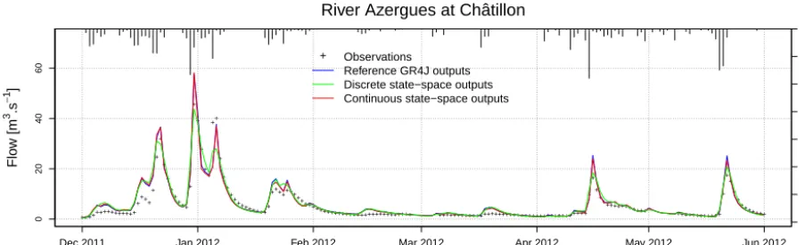
River Azergues at Châtillon
Figure 5.Simulated hydrograph of the River Azergues in the first half of 2012 during the validation period. The reference GR4 model (output in blue), the GR4 discrete state-space solution (output in green) and the continuous state-space solution (output in red) were calibrated with
C2M( √
Q)as the objective function.
in Table 3. With the continuous state-space model, we veri-fied the stability of the parameters. This stability is very im-portant for designing a model that is not dependent on its time step.
4 Results and discussion
4.1 Comparison of tested models at the daily time step Figure 4 shows that performances are globally similar among the different versions of the model with a calibration using the C2M on square-rooted flows. The performances of the
reference model and the continuous state-space solution are also similar after calibration with the two other transforma-tions of the flow in the objective function (not shown). In the case of the discrete state-space solution, the model does not seem to be able to reproduce high flows well but performs better on low flows than the two other models when the
ob-jective function used is theC2M with logarithmic
transfor-mation.
The study of the hydrographs provides complementary information. The reference GR4 model and the continuous space solution are very similar while the discrete state-space solution simulates lower peak flows (see example hy-drograph in Fig. 5). This behaviour can be explained because solving the 11 linear stores introduces errors that propagate and amplify across the Nash cascade.
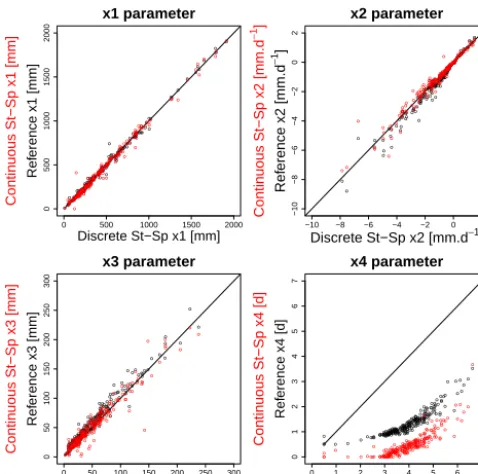
To extend the analysis on the similarity of the models, we compared the parameter values obtained by calibration. As shown in Fig. 6, the parameters have the same range of values. We can still note differences in the values of thex4
● ● ● ● ● ● ●● ● ● ● ● ● ● ● ● ● ● ● ● ● ● ● ● ● ● ● ● ● ● ● ● ● ● ● ● ● ● ● ● ● ● ● ● ● ●●●● ● ● ● ● ● ● ● ● ● ● ● ● ●●●●● ● ● ● ● ● ● ●● ● ● ● ● ● ● ● ● ● ●● ● ● ● ● ● ● ● ● ● ● ● ● ● ● ● ● ● ●● ● ● ●● ● ● ●● ● ● ● ● ● ● ● ● ● ● ● ● ● ● ● ● ● ●● ● ●● ● ● ● ● ● ● ● ● ● ● ● ● ● ● ● ●● ● ● ● ● ● ● ● ● ●● ● ●● ● ● ● ● ● ● ● ●● ●●● ● ● ● ●● ● ● ● ● ● ● ● ● ● ● ● ● ● ● ● ● ● ● ● ● ● ● ● ● ● ● ● ● ● ● ● ● ● ● ● ● ● ● ● ● ● ● ● ● ● ● ● ● ● ● ● ● ● ● ●
0 500 1000 1500 2000
0 500 1000 1500 2000 x1 parameter
Discrete St−Sp x1 [mm]
Ref
erence x1 [mm]
● ● ● ● ● ● ●● ● ● ● ● ● ● ● ● ● ● ● ● ● ● ● ● ● ● ● ● ● ● ● ● ● ● ● ● ● ● ● ● ● ● ● ● ● ● ● ●● ● ● ● ● ● ● ● ● ● ● ● ● ●● ● ● ● ● ● ● ● ● ● ●● ● ● ● ● ● ● ● ● ● ●● ● ● ● ● ● ● ● ● ● ● ● ● ● ● ● ● ● ●● ● ● ●● ● ● ●● ● ● ● ● ● ● ● ● ● ● ● ● ● ● ● ● ● ● ● ● ●● ● ● ● ● ● ● ● ● ● ● ●● ● ● ● ● ● ● ● ● ● ● ● ● ●●● ● ●● ● ● ● ● ● ● ● ● ● ●●● ● ●● ●● ● ● ● ● ● ● ● ● ● ● ● ● ● ● ● ● ● ● ● ● ●● ● ● ●● ● ● ● ● ● ● ● ● ● ● ● ● ● ● ● ● ● ● ● ● ● ● ● ● ● ● ● ● ● Contin
uous St−Sp x1 [mm]
●● ● ● ● ●● ● ● ● ● ● ● ● ● ● ● ● ● ● ● ● ● ● ● ● ● ● ● ● ● ● ● ● ● ● ● ● ● ●● ● ● ● ● ● ● ● ● ● ● ● ● ● ● ● ● ● ● ● ● ● ● ● ●● ● ● ● ●● ● ● ● ● ● ● ● ● ● ● ● ●● ● ● ● ● ● ●● ● ● ● ● ● ● ● ●● ● ● ● ●● ●● ● ● ● ● ● ● ● ● ● ● ● ● ● ● ● ● ● ● ● ● ● ● ● ● ● ● ● ● ● ● ● ● ● ●● ● ● ● ● ● ● ● ● ● ● ● ● ● ● ● ● ● ● ● ● ● ● ● ● ● ● ● ● ● ● ● ● ● ● ● ● ● ● ● ● ● ● ● ● ● ● ● ● ● ● ● ● ● ● ● ● ● ● ● ● ● ● ● ● ● ● ● ● ● ● ● ● ● ● ● ● ● ● ● ● ● ● ● ● ● ● ● ● ●
−10 −8 −6 −4 −2 0 2
−10 −8 −6 −4 −2 0 2 x2 parameter ●● ● ● ● ●● ● ● ● ● ● ● ● ● ● ● ● ● ● ● ● ● ● ● ● ● ● ● ● ● ● ● ● ● ● ● ● ● ●● ● ● ● ● ● ● ● ● ● ● ● ● ● ● ● ● ● ● ● ● ● ● ● ●● ● ● ● ● ● ● ● ● ● ● ● ● ● ● ● ● ●● ● ● ● ● ● ●● ● ● ● ● ● ● ● ●● ● ● ● ●● ●● ● ● ● ● ● ● ● ● ● ● ● ● ● ● ● ● ● ● ● ● ● ● ●● ● ● ● ● ● ● ● ● ● ●● ● ● ● ● ● ● ● ● ● ● ● ● ● ● ● ● ● ● ● ● ● ● ● ● ● ● ● ● ● ● ● ● ● ● ● ● ● ● ● ● ● ● ● ● ● ● ● ● ● ● ● ● ● ● ● ● ● ● ● ● ● ● ● ● ● ● ● ● ● ● ● ● ● ● ● ● ● ● ● ● ● ● ● ● ● ● ● ● ● ●
Discrete St−Sp x2 [mm.d−1]
Ref erence x2 [mm. d − 1] Contin uous St−Sp x2 [mm. d − 1] ● ● ● ● ● ● ● ● ● ● ● ● ● ● ● ● ● ● ● ● ●● ● ● ● ●●● ●● ● ● ● ● ● ●● ● ● ● ● ● ● ● ● ● ● ● ● ● ●● ● ● ● ● ● ● ● ● ● ● ●● ● ● ● ● ● ● ● ● ● ● ● ● ●● ● ● ● ● ● ● ● ● ● ● ● ● ● ● ●● ● ● ● ● ●●● ● ● ● ● ●● ● ● ● ● ● ● ● ● ● ● ● ● ● ● ● ● ● ● ● ● ● ● ● ● ● ● ● ● ● ● ● ● ● ● ● ● ● ● ● ● ● ● ● ● ● ● ● ● ● ● ● ● ● ●● ● ● ● ● ● ● ● ● ● ● ● ● ● ● ●● ● ● ● ● ● ● ● ● ● ● ● ● ● ● ● ● ●● ● ● ● ● ● ● ● ● ● ● ● ● ● ● ● ● ● ● ● ● ● ● ● ● ● ● ● ● ● ● ● ● ● ● ● ● ● ● ● ● ● ●
0 50 100 150 200 250 300
0 50 100 150 200 250 300 x3 parameter
Discrete St−Sp x3 [mm]
Ref
erence x3 [mm]
● ● ● ● ● ● ● ●● ● ● ● ● ● ● ● ● ● ● ● ●● ● ● ● ●●● ●● ● ● ● ● ● ●● ● ● ● ● ● ● ●● ● ● ● ● ● ●● ● ● ● ● ● ● ● ● ● ● ●● ● ● ● ● ● ● ● ● ● ● ● ● ● ● ● ● ● ● ● ● ● ● ● ● ● ● ● ● ●● ● ● ● ● ● ● ● ● ● ●●●●● ● ● ● ● ● ● ● ● ● ● ● ● ● ● ● ● ● ● ● ● ● ● ● ● ● ● ● ● ● ● ● ● ●● ● ● ● ● ● ● ● ● ● ● ● ● ●● ● ● ● ● ●● ● ● ● ● ● ● ● ● ● ● ●● ● ● ●● ● ● ● ● ● ● ●● ● ● ● ● ● ● ● ● ●● ● ● ● ● ● ● ● ● ● ● ● ● ● ● ● ● ● ● ● ● ● ● ● ● ● ● ● ● ● ● ● ● ● ● ● ● ● ● ● ● ● ● Contin
uous St−Sp x3 [mm]
● ● ● ● ● ● ● ● ● ● ● ●● ● ● ● ● ● ● ● ● ● ● ● ● ● ●●●●●● ● ● ● ● ● ● ● ● ● ● ● ● ● ● ● ● ● ● ● ● ● ● ● ● ● ● ● ● ● ● ● ● ● ● ● ● ● ● ● ● ● ● ● ●● ● ● ● ● ● ●● ● ● ● ●●● ● ● ● ● ● ●● ● ● ● ● ● ● ● ● ● ● ● ● ● ● ● ● ● ● ● ● ● ●● ● ● ● ● ● ● ● ● ● ●●●●●● ● ● ● ● ● ● ● ● ● ● ● ●● ● ● ● ● ● ● ● ● ●● ●● ● ●● ● ● ● ● ● ● ● ● ● ● ● ● ● ● ● ● ● ● ● ● ●● ● ● ● ● ● ●●● ● ● ● ● ● ●● ● ● ● ●●●● ●●● ● ● ●●●●●● ● ● ● ● ● ● ● ● ● ●● ● ● ● ● ● ● ● ● ● ●
0 1 2 3 4 5 6 7
0 1 2 3 4 5 6 7 x4 parameter
Discrete St−Sp x4 [d]
Ref
erence x4 [d]
● ● ● ● ● ● ● ● ● ● ● ● ● ● ● ● ● ● ● ● ● ● ● ● ● ● ● ● ● ● ● ● ● ● ● ● ● ● ● ● ● ● ● ● ● ● ● ● ● ●●● ● ● ● ● ● ● ● ● ● ● ● ● ● ● ● ● ● ● ● ● ● ● ●●● ● ● ● ● ● ●● ● ● ● ● ● ● ● ● ● ● ● ● ● ● ● ● ● ● ● ● ● ● ● ● ● ● ● ● ● ● ● ● ● ●● ● ● ● ● ● ● ● ● ● ● ●●● ● ● ● ● ● ● ● ● ● ● ● ● ● ● ●● ● ● ● ● ● ● ● ● ●● ●● ● ●● ● ● ● ● ● ● ● ● ● ● ● ● ● ● ● ● ● ● ● ● ● ● ●● ● ● ● ●●● ● ● ● ● ● ●● ● ● ● ● ●● ● ●● ● ● ● ● ● ● ● ● ● ● ● ● ● ● ● ● ● ● ●● ● ● ● ● ● ● ● ● ● ● Contin
uous St−Sp x4 [d]
Figure 6.Scatter plots of the four free parameters of the different versions of the models obtained by calibration withC2M(
√
Q)as
an objective function on the basins of the data set. Parameter com-parison between unit hydrograph and Nash cascade is in black and parameter comparison between discrete and continuous state-space parameters is in red. The values ofx1,x2andx3are similar for the models (the line represents they=xline). Thex4values are higher in the discrete state-space model than for the other model versions.
caused by unsuitable solving is confirmed by the fact that the x4 parameter values are similar for the three models at an
hourly time step (not shown here).
Last, to understand the internal impact of the state-space formulation on the model, we analysed state variables and internal fluxes. Two differences are induced by the model’s state-space formulation. First, the discrete Nash cascade out-put peaks are lower than the peaks of the unit hydrograph (Fig. 7). The peaks of the continuous state-space represen-tation are more similar with the reference but the peaks oc-cur sooner. The second difference between the models con-cerns the levels of the routing store (Fig. 8). Here we only compared the reference GR4 to the continuous state-space solution because the inputs in the routing store are too dif-ferent for the discrete state-space solution. The peak levels are higher in the continuous state-space representation, even sometimes higher than the maximum capacity of the rout-ing store. The reason for this is that we shifted from the dis-crete model in which the processes are treated sequentially to a continuous model in which all the processes are solved simultaneously. In the discrete model, the exchanges are first calculated based on the routing level at the beginning of the time step, then the output of the unit hydrograph is added and last the outflow of the routing store is calculated. Due to
this sequential treatment, in high-flow conditions, the quan-tity of exchanged water and the outflow of the routing store in the discrete model are lower than those of the continu-ous state-space representation. Given that most of the time the exchange parameter is negative, the lower outflow of the routing store is compensated for by less water loss with the groundwater exchange in the complementary flow branch. This can explain why the simulated flows are similar despite these internal differences.
Moreover, by analysing the differences between the two models, it is also important to take into account the computa-tional time. Indeed, running the original model version is on average 3 times faster than the continuous state-space ver-sion due to the adaptive sub-step method. This is important to consider for some applications.
This computational time rise is essentially due to the adap-tive sub-step algorithm. For example, in the River Azergues at Châtillon catchment, the mean number of sub-steps is 22 and it can reach 100 during some days. However, in Sect. 3.1 we argue that the adaptive sub-step method seems necessary to avoid numerical errors.
To conclude with these results, we can argue that the mod-ifications brought by the continuous state-space representa-tion, although they modify the model’s internal fluxes, do not degrade the model’s performance, but only slightly mod-ify the model’s internal fluxes. It is important to underline that the OS solving of a Nash cascade creates more errors than a discrete unit hydrograph. To be equivalent to the ref-erence model, the state-space representation of GR4 needs to be solved with a robust numerical technique.
4.2 Consistency of the state-space representation through time steps
The analysis of temporal consistency provides the most valu-able result produced by the continuous state-space represen-tation. The work of Ficchí et al. (2016) resulted in a GR4 model that is nearly consistent across time steps. However, to adapt the model, they chose to include the time step variations in a theoretical transformation between the free parameter values and the percolation fixed coefficient (Ta-ble 3) at different time steps. In this section, we only com-pare the reference GR4 with the continuous solution of the state-space representation. The parameters of the state-space representation discrete solution show the same behaviour as the reference GR4 ones so it was chosen not to show them. This proves that all the improvements shown in this section are only due to the continuous resolution of the state-space model.
Date
Input in the routing store [mm.d
−
1 ]
Dec 2011 Jan 2012 Feb 2012 Mar 2012 Apr 2012 May 2012 Jun 2012
0
5
10
15
20
140
120
100
80
60
40
20
0
Rainf
all [mm.d
−
1 ]
Reference GR4
Discrete state−space response Continuous state−space response
River Azergues at Châtillon
Figure 7.Daily inputs in the routing store of the River Azergues in the first half of 2012. The models are calibrated with theC2M( √
Q)as
the objective function. The peaks are lower with the discrete state-space GR4 (green lines) and occur sooner with the continuous state-space GR4 (red lines).
Date
Le
v
el of the routing store [mm]
Dec 2011 Jan 2012 Feb 2012 Mar 2012 Apr 2012 May 2012 Jun 2012
0
10
20
30
40
140
120
100
80
60
40
20
0
Rainf
all [mm.d
−
1 ]
Reference GR4J routing store level Continuous state−space routing store level
River Azergues at Châtillon
Figure 8. Daily routing store filling of the River Azergues in the first half of 2012. The reference GR4 (blue line) and the continuous state-space representation (red line) are calibrated with theC2M
√
Qas the objective function.
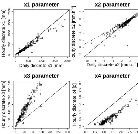
between the two time steps but it is important to note that the values of thex3parameter follow the relations proposed
by Ficchí et al. (2016) (the dashed lines). The high values of x1are underestimated compared to the theoretical relation as
are the low values of thex2parameter. There is also an issue
with the unit hydrograph parameter (x4in Fig. 9) for which
calibrated hourly parameter values are systematically lower than the values it would have by following the transforma-tion. Kavetski et al. (2011) and Littlewood and Croke (2008) encountered the same issue with the lag parameter of their models.
The values of x1, x2 and x4 are inconsistent compared
to the values expected using the theoretical transformations. Regarding the work of Ficchí (2017), we can argue that the changes in the high values of x1 and the low values of x2
are due to temporal inconsistencies in the interception cal-culation. The case of thex4parameter is more problematic.
The differences in thex4values probably stem from the
dis-cretization of the unit hydrograph at different time steps.
In the continuous state-space model, the time step is taken into account in the temporal numerical integration of the model. For this reason, in theory there is no need to adapt the values of the parameters. This is confirmed in Fig. 10, where the values of calibrated parameters remain approxi-mately constant despite the time step change. Only the high values ofx1and the values ofx2slightly diverge from the
x=yline.
This result is useful in building a model that can adapt its time step resolution depending on the given conditions. The results are particularly interesting for the case of x4
values because thex4 values are constant between the two
● ● ● ● ● ● ● ● ● ● ● ● ● ● ● ●● ● ● ● ● ●● ● ● ● ● ● ● ● ● ● ● ● ● ● ● ● ● ● ● ● ● ● ● ● ●●●● ● ● ● ● ● ● ● ● ● ● ●●●●●●● ● ● ● ●● ● ● ● ● ● ● ● ●● ● ● ●●● ● ● ● ● ● ● ● ● ● ● ● ●● ● ● ● ● ●●● ● ● ●● ● ● ●● ● ● ● ● ● ● ● ● ● ● ● ● ● ● ● ● ● ●● ● ●● ● ● ● ●● ● ● ● ● ●● ● ● ● ● ●● ● ● ● ● ● ● ● ● ●● ● ●● ● ●● ●● ● ● ●● ● ●● ● ● ● ● ● ● ● ● ● ● ● ● ● ● ● ● ●● ● ● ● ● ● ● ● ● ● ● ● ● ● ● ● ● ● ● ● ● ● ● ● ● ● ● ● ● ● ● ● ● ● ● ● ● ● ● ● ●● ●
0 500 1000 1500 2000
0 500 1000 1500 2000 x1 parameter
Daily discrete x1 [mm]
Hour
ly discrete x1 [mm]
●● ● ● ● ●● ● ● ● ●● ● ● ● ● ● ● ● ● ● ● ● ● ● ● ● ●● ● ● ● ● ● ● ● ● ● ● ●● ● ● ● ●● ● ● ● ● ● ● ● ● ● ● ● ● ● ● ● ●● ●●● ● ● ● ● ● ● ● ● ●● ● ● ● ● ● ● ●● ● ● ● ● ● ●● ● ● ● ●● ● ● ●● ● ● ●● ● ●● ●● ● ● ●● ● ● ● ● ● ● ● ● ●● ● ● ● ● ● ● ●● ● ● ● ● ●● ● ● ● ●● ● ● ● ● ●● ● ● ● ● ● ● ● ● ● ●●● ● ● ● ● ●● ● ● ● ● ● ● ● ● ● ● ● ● ● ● ● ● ● ● ● ● ● ● ● ● ● ● ● ● ● ● ● ● ● ● ● ● ● ● ● ● ● ● ● ● ● ● ● ● ● ● ● ● ● ● ● ● ● ● ● ● ● ● ● ●
−10 −8 −6 −4 −2 0 2
−10 −8 −6 −4 −2 0 2 x2 parameter
Daily discrete x2 [mm.d−1]
Hour ly discrete x2 [mm. h − 1 ] ● ● ● ● ● ● ● ● ● ● ● ● ● ● ● ● ● ● ● ● ● ● ● ● ● ●●● ●● ● ● ● ● ● ● ● ● ● ● ● ● ● ● ● ● ● ● ● ● ●● ● ● ● ● ● ● ● ● ● ● ● ● ● ● ● ● ● ● ● ● ● ● ● ● ● ● ● ● ● ● ● ● ● ● ● ● ● ● ● ● ● ● ● ● ● ● ● ● ● ● ● ● ● ● ● ●● ●● ● ● ● ● ● ● ● ● ● ● ● ● ● ● ● ● ● ● ● ● ● ● ● ● ● ● ● ●● ● ● ● ● ● ● ● ● ● ● ● ● ● ● ● ● ● ● ● ● ● ● ● ● ● ● ● ● ● ● ● ● ● ● ● ● ●● ● ● ●● ● ● ● ● ● ● ● ● ● ● ● ● ●● ● ● ● ● ● ● ● ● ● ● ● ● ● ● ● ● ● ● ● ● ● ●● ● ● ● ● ● ● ● ● ● ● ● ● ● ● ● ● ● ● ●
0 50 100 150 200 250 300
0 50 100 150 200 250 300 x3 parameter
Daily discrete x3 [mm]
Hour
ly discrete x3 [mm]
● ● ● ● ● ● ● ● ●● ● ● ● ● ● ● ● ● ● ● ● ● ● ● ● ●●● ● ● ● ● ● ● ● ● ● ● ●● ● ● ● ● ● ● ● ● ●● ● ● ●● ● ●● ● ● ● ● ● ● ● ● ● ● ● ● ● ● ● ● ●● ● ● ● ● ● ●● ● ● ● ●●● ● ● ● ● ● ● ● ● ● ● ● ● ● ● ● ● ● ● ● ● ● ● ● ● ● ● ●●●● ● ● ● ●● ● ● ● ● ● ●● ●● ● ● ● ● ● ● ● ● ● ● ● ● ● ● ●● ● ● ● ● ● ● ● ● ● ● ● ●● ● ● ● ● ● ● ● ● ● ● ● ● ● ● ● ● ● ● ● ● ● ● ● ● ● ● ● ● ● ● ●● ● ● ● ●● ● ● ●●●● ● ●●● ● ● ● ● ● ● ● ● ● ●● ●● ● ● ● ● ● ● ● ● ● ● ● ● ● ●● ●
0.0 0.5 1.0 1.5 2.0 2.5 3.0
0.0 0.5 1.0 1.5 2.0 2.5 3.0 x4 parameter
Daily discrete x4 [d]
Hour
ly discrete x4 [d]
Figure 9.Scatter plots representing the four parameters of the ref-erence (daily and hourly) GR4 models obtained by calibration with
C2M(√Q)as the objective function. The solid line represents the
y=xregression and the dashed lines the transformation relations of Table 3.
● ● ● ● ● ● ● ● ● ● ● ● ● ● ● ●●● ● ● ● ●● ● ● ● ● ● ● ● ● ● ● ● ● ● ● ● ● ● ● ● ●● ● ● ●●●● ● ● ● ● ● ● ● ● ● ● ●● ●●●●● ● ● ● ●● ● ● ● ● ●● ● ●● ● ● ● ●● ● ● ● ● ● ● ● ● ● ● ● ● ● ● ● ● ● ●● ● ● ● ●●● ● ●● ● ● ● ● ● ● ● ● ● ● ● ● ● ● ● ● ● ●● ● ●● ● ● ● ● ● ● ● ● ● ●● ● ● ● ● ● ● ● ● ● ● ● ● ● ●●● ● ●● ● ● ● ●● ● ● ●● ●●● ● ●● ●● ● ● ● ● ● ● ● ● ● ● ● ●● ● ● ● ● ● ● ● ●● ● ● ● ● ● ● ● ● ● ● ● ● ● ● ● ● ● ● ● ● ● ● ● ● ● ● ● ● ● ● ●● ●
0 500 1000 1500 2000
0 500 1000 1500 2000 x1 parameter
Daily state−sp x1 [mm]
Hour
ly state−sp x1 [mm]
●● ● ● ● ●● ● ● ● ●● ● ● ● ● ● ● ● ●● ● ● ● ● ● ● ● ● ● ● ● ● ● ● ● ● ● ●● ● ● ● ● ● ● ● ● ● ● ● ● ● ● ● ● ● ● ● ● ● ● ● ● ●● ● ● ● ● ● ● ● ● ● ● ● ● ● ● ● ● ● ● ●● ● ● ● ● ● ●● ● ● ● ●●● ● ● ● ● ● ● ● ● ● ● ● ● ● ● ● ● ● ● ● ● ● ● ● ● ●● ● ● ● ● ● ● ● ● ● ● ● ● ● ● ● ● ● ● ●● ● ● ● ● ●● ● ● ● ● ● ● ● ● ● ● ● ● ● ● ● ● ● ● ● ● ● ● ● ●● ● ● ● ● ● ● ● ● ● ● ● ● ● ● ● ● ● ● ● ● ● ● ● ● ● ● ● ● ● ● ● ● ● ● ● ● ● ● ● ● ● ● ● ● ● ● ● ● ● ● ● ● ● ● ● ● ● ●
−10 −8 −6 −4 −2 0 2
−10 −8 −6 −4 −2 0 2 x2 parameter
Daily state−sp x2 [mm.d−1]
Hour ly state−sp x2 [mm. d − 1 ] ● ● ● ● ● ● ● ●● ● ● ● ● ● ● ● ● ● ● ● ● ● ● ● ● ●●●●● ● ● ● ● ● ●● ● ● ● ● ● ● ●● ● ● ● ●●●● ● ● ● ● ● ● ●● ● ● ●● ● ● ● ● ● ● ● ● ● ● ● ● ●● ● ● ● ● ● ● ● ● ● ● ● ● ● ● ●● ● ● ● ● ● ● ● ● ● ●● ● ● ● ●●● ● ● ● ● ● ● ● ● ● ● ● ● ● ● ● ●● ● ● ● ● ● ● ● ● ● ● ● ● ●● ● ● ● ● ● ● ● ● ● ● ● ● ●● ● ● ●● ●●● ● ● ● ● ● ● ● ● ●●● ●●●● ● ●●●● ●●● ● ● ● ● ● ● ● ● ● ● ● ● ● ● ● ● ● ●● ● ● ● ● ● ● ● ● ● ● ● ● ● ●● ● ● ● ● ● ● ● ● ● ●● ● ● ● ● ● ● ●
0 50 100 150 200 250 300
0 50 100 150 200 250 300 x3 parameter
Daily state−sp x3 [mm]
Hour
ly state−sp x3 [mm]
● ● ● ● ● ● ● ● ●● ● ● ● ● ● ● ● ● ● ● ● ● ● ● ● ●●●● ● ● ● ●● ● ● ● ● ● ● ● ● ● ● ● ● ● ● ● ●● ● ● ● ● ● ● ● ● ● ● ● ● ● ● ● ● ● ● ● ● ● ● ● ● ● ● ● ● ● ● ● ● ● ● ● ● ●●● ● ● ● ● ● ● ● ● ● ● ● ● ● ● ● ● ● ● ● ● ● ● ● ● ● ● ●●● ● ● ● ● ● ● ● ● ● ● ● ● ● ●● ● ● ● ● ● ● ● ● ● ● ● ● ● ● ●● ● ● ● ● ● ● ●● ● ● ● ●● ● ● ● ● ● ● ● ●● ● ● ● ● ● ● ● ● ● ● ● ● ● ● ● ● ● ● ● ● ●●● ● ●● ● ● ● ● ● ● ● ● ● ●● ● ● ● ●● ● ● ● ● ● ●● ● ● ● ● ● ● ● ● ● ●● ● ● ● ● ●● ●
0.0 0.5 1.0 1.5 2.0 2.5 3.0
0.0 0.5 1.0 1.5 2.0 2.5 3.0 x4 parameter
Daily state−sp x4 [d]
Hour
ly state−sp x4 [d]
Figure 10.Scatter plots representing the four parameters of the con-tinuous state-space (daily and hourly) GR4 models obtained by cal-ibration withC2M(√Q) as the objective function. The solid line represents they=xline.
work on a wide range of catchments. However, in addition to the input errors, the lack ofx4time consistency can also be
explained by the integration errors produced by the OS at a daily time step.
The outliers in x3 values that occur in Fig. 10 are also
present in Fig. 9. No explanations relating to physical charac-teristics of these catchments or simulation performance were found. We assume that these outlier values are due to the non-sensitivity of thex3parameter for these catchments.
Finally, to verify stability, we also need to compare the performance of the models at the hourly time step. Figure 11 shows that, as at the daily time step, the performance is sim-ilar for the different versions.
Thus, the continuous state-space representation shows bet-ter temporal stability in thex4parameter values with similar
performance.
5 Conclusions and perspectives
The objective of this study was to present a version of a bucket-type rainfall–runoff model with a robust numerical resolution of the governing water balance equations by set-ting up a continuous state-space representation. The method-ology is based on (i) identifying the state variables, (ii) writ-ing their differential equations, (iii) replacwrit-ing certain compo-nents of the model with more easily described compocompo-nents in terms of differential equations (namely replacing the unit hydrograph with a Nash cascade here), and (iv) solving these equations with a robust numerical integration technique. Fi-nally, all the fluxes that form the water balance equation gov-erning a state are solved simultaneously while they are solved sequentially in OS models. As stated by Fenicia et al. (2011), this is more physically satisfying.
This work was presented using the example of the GR4 model. The new version was created to be as close as possi-ble to the initial model but a single modification was imple-mented: a Nash cascade substitutes the model’s unit hydro-graph.
When analysing the results and the output flows, it was shown that the new formulation, when solved with a robust numerical technique, has a limited impact on performance. However, the analysis of the parameter values and of the internal fluxes of the model shows that some discrepancies occur when running the model. The peak flow of the Nash cascade occurs sooner than the peak flow of the unit hy-drograph. The amount of water in the routing store and ex-changed by the groundwater exchange function is also higher for the state-space representation, particularly during high-flow periods.
More-●● ● ● ●
●
●● ● ● ●● ●
●
●● ●
● ● ● ● ●
●
Reference St−Sp
disc
St−Sp cont C2M
(
Q
) ● ● ●
0.0
0.2
0.4
0.6
0.8
1.0
● ●
● ● ●
● ●
● ●
● ●●
● ● ●
● ●
● ●
● ●●
● ● ●
● ● ● ●
●
Reference St−Sp
disc
St−Sp cont C2M
(
Q
)
● ● ●
0.0
0.2
0.4
0.6
0.8
1.0
Reference St−Sp
disc
St−Sp cont C2M
(
log
(
Q
))
● ● ●
0.0
0.2
0.4
0.6
0.8
1.0
(a) (b) (c)
Figure 11.Performance comparisons obtained in validation among the reference (with unit hydrograph), the discrete state-space (with Nash cascade) and the continuous state-space hourly GR4 on 240 catchments, focusing on high (a), intermediate(b)and low (c)flows after calibration with theC2M(√Q)(i.e. focusing on intermediate flow). The points represent the mean performance.
over, the use of the Nash cascade rather than the unit hy-drograph improves (when solved with implicit Euler) the lag parameter value stability with time steps. This improved sta-bility can make it easier to calibrate the model with a given data set and to apply it at a finer time step for which no dis-charge data are available. It can also allow the use of a model that runs at a finer time step in high-flow periods and a larger time step in low-flow periods.
Furthermore, the comparison between the discrete and continuous state-space model shows that the benefits pro-vided by the continuous state-space representation are a re-sult of the use of a robust numerical integration technique. Indeed, solving the state-space representation using OS in-troduces errors that impact the simulated flow values and do not result in parameter stability. Thus, the real benefit of the use of the Nash cascade is to simplify the numerical solving application.
The performance obtained with the continuous state-space model is not better than that of the original model. In addi-tion, because the number of sub-steps sometimes needs to be high, the computational time is longer with the continu-ous state-space representation of the model. Consequently, the use of this representation would be helpful for particular applications such as time-variable modelling. It might also be useful for certain data assimilation techniques (typically vari-ational methods) because all the components are represented as states and the governing equations are clearly defined.
In addition, it could also be advantageous to find a way to adapt the number of stores of the Nash cascade to the catch-ment studied.
Although it is necessary to adapt the Nash cascade to dif-ferent unit hydrograph shapes, this article suggests a suf-ficiently general methodology to erase OS in hydrological bucket-type modelling and can be transposed to other mod-els.
Code and data availability. The Fortran code used in this arti-cle can be freely downloaded from GitHub at https://github.com/ HYDRO-group-Irstea-Antony/GR4-State-space-version-1.0 (last access: 18 April 2018). The state-space model can be tested on an example catchment data set with already calibrated model pa-rameters. The full reference for this code can be found in the ref-erences (Santos, 2017); it is referenced with the following DOI: https://doi.org/10.5281/zenodo.1118183.
Author contributions. This work is part of LS’ PhD work; he made the technical development and the analysis and wrote the paper. GT and CP are the PhD supervisors; they supervised this work and the paper writing.
Competing interests. The authors declare that they have no con-flicts of interest.
Acknowledgements. The first author’s PhD grant was provided by Irstea. We thank Météo France for providing the SAFRAN climatic data used in this work. We also would like to thank Martyn Clark for his advice in setting-up the differential equations, Nicolas Le Moine for sharing his ideas to replace the unit hydrographs and on the nu-merical integration, Fabrizio Fenicia for his advice on nunu-merical integration and Paul-Henry Cournède for his analysis of the math-ematical adequacy of the model. Finally, we give special thanks to Andrea Ficchí for his work on the database and for the discussions on the temporal stability of the GR4 model.
We thank the topical editor, Jeffrey Neal, for his monitoring of the review process and his relevant reviewers choice. We also acknowledge the two reviewers, Barry Croke, and the anonymous reviewer for their very interesting and complementary remarks.
Edited by: Jeffrey Neal