www.geosci-model-dev.net/10/239/2017/ doi:10.5194/gmd-10-239-2017
© Author(s) 2017. CC Attribution 3.0 License.
A high-fidelity multiresolution digital elevation model
for Earth systems
Xinqiao Duan1,2, Lin Li1,3,4, Haihong Zhu1,4, and Shen Ying1,4
1Geographical Information Science Faculty, SRES School, Wuhan University, Wuhan 430079, China 2Hubei Geomatics Information Centre, Wuhan 430074, China
3Geospatial Information Science Collaborative Innovation Centre of Wuhan University, Wuhan 430079, China 4The Key Laboratory for Geographical Information System, Ministry of Education, Wuhan 430079, China Correspondence to:Lin Li ([email protected])
Received: 3 March 2016 – Published in Geosci. Model Dev. Discuss.: 27 May 2016 Revised: 8 November 2016 – Accepted: 21 December 2016 – Published: 16 January 2017
Abstract.The impact of topography on Earth systems vari-ability is well recognised. As numerical simulations evolved to incorporate broader scales and finer processes, accurately assimilating or transforming the topography to produce more exact land–atmosphere–ocean interactions, has proven to be quite challenging. Numerical schemes of Earth systems often use empirical parameterisation at sub-grid scale with down-scaling to express topographic endogenous processes, or rely on insecure point interpolation to induce topographic forc-ing, which creates bias and input uncertainties. Digital ele-vation model (DEM) generalisation provides more sophis-ticated systematic topographic transformation, but existing methods are often difficult to be incorporated because of un-warranted grid quality. Meanwhile, approaches over discrete sets often employ heuristic approximation, which are gener-ally not best performed. Based on DEM generalisation, this article proposes a high-fidelity multiresolution DEM with guaranteed grid quality for Earth systems. The generalised DEM surface is initially approximated as a triangulated ir-regular network (TIN) via selected feature points and possi-ble input features. The TIN surface is then optimised through an energy-minimised centroidal Voronoi tessellation (CVT). By devising a robust discrete curvature as density function and exact geometry clipping as energy reference, the devel-oped curvature CVT (cCVT) converges, the generalised sur-face evolves to a further approximation to the original DEM surface, and the points with the dual triangles become spa-tially equalised with the curvature distribution, exhibiting a quasi-uniform high-quality and adaptive variable resolution. The cCVT model was then evaluated on real lidar-derived
DEM datasets and compared to the classical heuristic model. The experimental results show that the cCVT multiresolution model outperforms classical heuristic DEM generalisations in terms of both surface approximation precision and surface morphology retention.
1 Introduction
1.1 Topography in Earth systems
Topography is one of the main factors controlling processes operating at or near the surface layer of the planet (Florin-sky and Pankratov, 2015; Wilson and Gallant, 2000). With the success of Earth and environment systems with these scale-diversified processes, persistent demands exist for ex-tending their utility to new and expanding scopes (Ringler et al., 2008; Tarolli, 2014; Wilson, 2012), as exemplified by lapse-rate-controlled functional plant distributions (Ke et al., 2012), orographic forcing imposed on oceanic and atmo-spheric dynamics (Nunalee et al., 2015; Brioude et al., 2012; Hughes et al., 2015), topographic dominated flood inunda-tions (Bilskie et al., 2015; Hunter et al., 2007), and many other geomorphological (Wilson, 2012), soil (Florinsky and Pankratov, 2015), and ecological (Leempoel et al., 2015) examples from Earth systems. However, as numerical sim-ulation systems evolved to incorporate broader scales and finer processes to produce more exact predictions (Ringler et al., 2011; Weller et al., 2016; Wilson, 2012; Zarzycki et al., 2014), how to accurately assimilate or transform the
240 X. Duan et al.: A high-fidelity multiresolution DEM for Earth systems
resolution topography has proven to be a quite difficult task (Bilskie et al., 2015; Chen et al., 2015; Tarolli, 2014).
Earth and environmental simulations usually adopt sub-grid schemes to express topography heterogeneity processes (Fiddes and Gruber, 2014; Kumar et al., 2012; Wilby and Wigley, 1997). The sub-grid schemes are designed for the empirical parameterisation rather than accurate topography representation, which often leads to mixed-up uncertainties and bias of endogenous variability (Jiménez and Dudhia, 2013; Nunalee et al., 2015). However, under-resolved repre-sentation could be improved by variable-resolution enhance-ment, and bias of simulations can be justified by more fidelity topography transformation (Nunalee et al., 2015; Ringler et al., 2011). Topography is also commonly treated as a static boundary layer in dynamics simulations, where different in-terpolation strategies and mesh refinement techniques are used to convey terrain variation (Guba et al., 2014; Kesser-wani and Liang, 2012; Nikolos and Delis, 2009; Weller et al., 2016). But a mesh constructed from interpolated vertices does not necessarily comply with the terrain relief, and ele-vation errors are frequently reported as an input uncertainty (Bilskie and Hagen, 2013; Hunter et al., 2007; Nunalee et al., 2015; Wilson and Gallant, 2000). Although there are many situations where dynamic conditions are stressed as stronger impacts on predictions (Cea and Bladé, 2015; Budd et al., 2015), the underlying topography is still very impor-tant due to its increasingly improved fidelity to the Earth’s surface (Bates, 2012; Tarolli, 2014), and a sophisticated to-pography transformation would be beneficial to reduce dis-crepancies arising from physical inconsistencies (Chen et al., 2015; Glover, 1999; Ringler et al., 2011).
1.2 Multiresolution DEM
Systematic scale transformation of topographic data has long been studied under terrain generalisation, where precise sur-face approximation and terrain structural feature retention have both been pursued (Ai and Li, 2010; Chen et al., 2015; Guilbert et al., 2014; Jenny et al., 2011; Weibel, 1992; Zhou and Chen, 2011). Triangulated irregular networks (TINs) are generally chosen as a substitute for the regularly spaced grids (RSGs), and terrain feature points (critical points or salient points from some significance metric) are selected for con-structing the network. Triangular networks are used for their adaptiveness to locally enhanced multiresolution schemes. Critical points or salient points are selected because they can effectively improve the approximation precision (Heckbert and Garland, 1997; Zakšek and Podobnikar, 2005; Zhou and Chen, 2011).
As surface approximation precision and terrain feature retention are competitive for the redistribution of feature points, digital elevation model (DEM) generalisation is dif-ferentiated from terrain generalisation by its emphasis on surface approximation as a whole, with the aim of provid-ing precise surface interpolation (Guilbert et al., 2014).
Ter-rain generalisation emphasises geomorphology or landform depiction, where map generalisation measures (such as ab-stracting, smoothing) are drawn to produce progressive data reduction, with the effect that the main relief features are strongly stressed while non-structural details are massively suppressed (Ai and Li, 2010; Guilbert et al., 2014; Jenny et al., 2011). Since the static topographic layers are com-monly composed directly from DEM datasets for diverse simulation interests, maintaining precise surface approxima-tion for rigorous boundary condiapproxima-tions is often more important than “sparse” geomorphology representation. While DEM datasets are usually used interchangeably with topography or terrain in Earth systems, we will use DEMs and topography indiscriminately hereafter.
Existing DEM generalisations can be catalogued into two broad classes, namely, heuristic refinements and smooth fittings, according to differences in surface approximation strategy. The first class of approaches is due to the compu-tational feasibility consideration, for selecting a TIN surface that best approximates the original DEM surface from ex-haustively enumerating (of triangular combinations) requires exponential time (Chen and Li, 2012; Heckbert and Garland, 1997). It thus forces existing research to employ some heuris-tic strategy, in which insertion (or deletion) refinements on feature points are adopted, to find a sub-optimal approxi-mation that is computationally practical. In each insertion (or deletion), rearranging the entire existing grid to obtain a better approximation is also computationally prohibitive and thus not adopted (Chen et al., 2015; Heckbert and Garland, 1997; Lee, 1991); this may result in the clustering of feature points (Chen and Li, 2012). Among those existing heuris-tic approaches, trenching the pre-extracted terrain features (drainage streamlines, for example) into the TIN surface seems quite appealing (compound method) (Chen and Zhou, 2012; Zhou and Chen, 2011), but the quality of the gener-alised TIN surface cannot be guaranteed, and the existence of sliver triangles makes it difficult to be incorporated with sim-ulation numerical stability (Kim et al., 2014; Weller et al., 2009). The second class of approaches recognised the TIN surface constructed from locally computed feature points as not a good approximation to the original DEM surface. Much research thus considered global approximation instead of re-lying on an elaborate feature point selection scheme, such as bi-linear, bi-quadric, multi-quadric, Kriging, or general ra-dial base function-based fitting (Aguilar et al., 2005; Chen et al., 2015; Schneider, 2005; Shi et al., 2005). The pro-posed multi-quadric method (Chen et al., 2012, 2015), for example, well approximates the original DEM surface with a high-order smooth surface, and the smooth surface provides a kind of rejection mechanism to cure the feature point cluster-ing problem. However, the high-order radial base function is computationally expensive when a broad scenario is involved (Chen et al., 2015; Mitášová and Hofierka, 1993). In brief, existing DEM transformations are neither well performing,
with respect to loyalty to the original terrain surface, nor eas-ily incorporated by the numerical schemes.
1.3 Aims and contributions
The purpose of this article is to devise a multiresolution DEM that optimises surface approximation and guarantees grid quality that can be easily incorporated into the simu-lation systems. Multiresolution is an effective paradigm to model scale diversity (Du et al., 2010; Guba et al., 2014; Ringler et al., 2011; Weller et al., 2016). Amongst a number of promising approaches, we are especially fascinated by the centroidal Voronoi tessellations (CVTs) method as an intu-itive way to redistribute samples with a designated function (Du et al., 1999, 2010; Ringler et al., 2011) to develop an optimised surface transformation method to realise multires-olution terrain models.
CVT is essentially a two-step optimisation loop, i.e. spatial domain equalisation from Voronoi tessellation and property domain equalisation from barycentre computation (Du et al., 1999). To make this general optimisation method work for DEM transformation, we made the following contributions:
1. The generalised DEM surface is initially approximated by a triangular grid constructed from selected feature points. The selection of feature points have important morphological structures embedded (in the form of se-rialised points sequences) for computed (such as the D8 flow algorithm) or auxiliary input morphological lines, which have been proved to have a significant influence on the quality of the transformed DEM surface (Zhou and Chen, 2011). The proposed method keeps the struc-tural lines in the optimisation loop and makes it differ-ent to existing CVT implemdiffer-entations where stationary points are commonly not considered.
2. For the discrete TIN surface, we compute robust mean curvature on each facet. The attached curvature acts as a frequency distribution. In this discrete spatial domain and frequency domain, the CVT loops and makes sam-ple facets equalised from both domains. Spatial equal-isation warrants a quasi-uniform grid quality, while the curvature domain equalisation warrants adaptive distri-bution conforming to the terrain relief. It is thus a totally different DEM generalisation approach, and we called it curvature CVT (cCVT).
3. Existing CVT implementations often undertake a clus-tering approach. However, clusclus-tering over discrete sets suffers from numerical issues such as zigzag bound-aries, invalid cluster cells (Valette et al., 2008), and lim-ited grid quality. By devising an exact geometry clip-ping technique, this article develops a dedicated CVT algorithm for DEM transformation that helps to im-prove or avoid the numeric problems listed above.
The cCVT works on discrete sets but has a global opti-misation mechanism. It promises an optimised surface ap-proximation and quality grid, which can be used to build a high-fidelity multiresolution terrain model. From this ter-rain model, reliable surface variables can be estimated under a coupled system, or improved computational mesh can be constructed and refined to possible dynamic conditions. 1.4 Organisation of the article
The rest of the article is organised as follows. In Sect. 2, the theory behind CVT for optimised DEM surfaces is in-troduced, techniques for incorporating DEM generalisation principles and fast convergence are presented, and the differ-ences between the cCVT implementation and classical clus-tering approach are discussed. In Sect. 3, the cCVT model is tested with real lidar-derived terrain datasets. Section 4 discusses some considerations, comparable results, possi-ble causes, and interpretations of the cCVT model. Finally, Sect. 5 briefly presents a short conclusion and outlook.
2 Curvature centroidal Voronoi tessellation on DEM surface
2.1 Definition
Centroidal Voronoi tessellation is a space tessellation for each Voronoi cell’s geometrical centre (in the spatial domain) that coincides with its barycentre from the abstract property domain (Du et al., 1999). Here, the property domain is anal-ogous to the frequency domain. For the vertex sett{vi}1k in ⊂R3, the Voronoi tessellation graph is defined as Vi=p∈: |p−zi|<
p−vj
, j=1. . .k, j6=i , (1)
i=1. . .k.
Specifically, a Voronoi cellVi is the set of points whose
dis-tance tovi is less than that to any other vertices.| · |is the
Euclidean norm. Every vertex and its corresponding dual cell commonly have some intensity scalarρ attached from some abstract property domain, which is called a density function. The total potential energy of the Voronoi graphV of a ter-rain surface can be computed by summing up the potential energies of all cellsVi:
E= k
X
i=1
Z Z
ρ· |p−vi|2·dσ. (2)
The energy minimiser is x=
RR
x·ρ·dσ
RR
ρ·dσ ; y=
RR
y·ρ·dσ
RR
ρ·dσ ; z=
RR
z·ρ·dσ
RR
ρ·dσ , (3) which minimises the surface’s total potential, since vi= (x, y, z)satisfies
∂E
∂p =2(p−vi)·
Z Z
ρ·dσ=0. (4)
242 X. Duan et al.: A high-fidelity multiresolution DEM for Earth systems
In other words, when vi coincides with the barycentrevi,
each cell’s potential effect on the property domain (gravity) becomes equalised to a stable energy state.
2.2 Lloyd’s relaxation
The most classical energy minimisation process of cen-troidal Voronoi tessellation is expressed by Lloyd’s relax-ation (Lloyd, 1982). The main idea of this algorithm is to first tessellate the surface, and then perform density integra-tion over the area to find a “gravity” barycentre for each tes-sellated cell, which is used as the new site for the iteration. The pseudo-code of this procedure is shown below.
Algorithm 1Lloyd’s relaxation Inputs: vertex setN= {vi}1k while (1E >Threshold)
{
use the k vertices to tessellate the surface, obtain Voronoi cells{Vi};
clearN; for eachViin{Vi}
{
Compute barycentre ofVi:x= RR
x·ρ·dσ RR
ρ·dσ ;y= RR
y·ρ·dσ RR
ρ·dσ
z=
RR z·ρ·dσ RR
ρ·dσ ; push (xy)toN;
}
computeE;
}
We follow Lloyd’s elegant idea. The barycentre of a two-dimensional Voronoi cell may fall outside this surface patch, so an additional calculation may be needed. Du et al. (2003) suggested projecting the barycentre onto a nearest facet and using instead the constrained projection point for the new site. Others suggested quadric interpolations over all the facets of the cluster for more accurate site calculations (Valette et al., 2008).
2.3 Fast convergence to DEM equilibria 2.3.1 Clustering CVTs
Lloyd’s relaxation requires Voronoi tessellation on a discrete two-dimensional surface, but direct Voronoi tessellation on a piecewise smooth surface requires costly geodesic computa-tion and may be challenged by complicated numerical issues (Cabello et al., 2009; Kimmel and Sethian, 1998). Du et al. suggested that CVT could be realised through some cluster-ing approaches (Cohen-Steiner et al., 2004; Du et al., 1999, 2003), i.e. using the associated property as density function to cluster facets and then find the clustered cells’ barycentres to create new clustering sites. Through this heuristic itera-tion, the new sites along with the new tessellations compose
a better and better approximation to the original surface, with their spatial distribution conforming to the pre-defined den-sity function.
The clustering approach avoids geodesic tessellation by di-rect facet combination, which is computationally light. The greatest expenditure then comes from global distance com-putation for identifying every cell to its cluster centre. How-ever, this k-means like clustering over discrete facets suffers from some numeric issues, such as zigzag cluster cell bound-aries – since no geodesic Voronoi tessellation was used, and invalid clusters due to disconnected set of facets (Valette and Chassery, 2004; Valette et al., 2008). Furthermore, the key to the quick clustering algorithm is that it avoids generating new sites (to avoid surface reconstruction) and relies on ex-isting sites (or facets). Thus, the generated grid cells may not be well qualified.
2.3.2 Curvature as density function
Terrain surface critical points such as peaks, pits, and saddles are treated as gravity equilibria and key elements depicting the surface geometry in the large (Banchoff, 1967; Milnor, 1963); a further extension of the critical points on second-order surface derivatives will describe a more fundamental terrain geometry shape (Jenny et al., 2011; Kennelly, 2008). When constructing a generalised DEM surface, these feature points are commonly used as a base set, and additional in-put points, or pre-extracted terrain structures, are embedded for further approximation (Guilbert et al., 2014; Zakšek and Podobnikar, 2005; Zhou and Chen, 2011). The additional in-put points or pre-extracted terrain structures of interest are also commonly required in numerical simulation setups for cross-checking or validation purposes.
Based on these observations, and considering require-ments of the CVT variational framework, this article pro-poses a feature point-based scheme (including boundary points, feature points, and pre-extracted structural points of interest) as initial Voronoi sites. For optimised spatial tribution of these sample points, we calculate a robust dis-crete mean curvature as a density function, which is based on the recognition of curvature’s flexibility in capturing shape characteristics and capability in conducting shape evolution (Banchoff, 1967; Kennelly, 2008; Pan et al., 2012). Cur-vature’s ability to flexibly describe terrain morphology has been appreciated by many researchers. For example, Ken-nelly (2008) noted that, compared to the results of the flow accumulation model, curvature-based delineation of drainage networks is not limited to 1 pixel thickness and requires no depression filling. The robust discrete curvature calculation is referred to in Meyer et al. (2003).
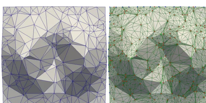
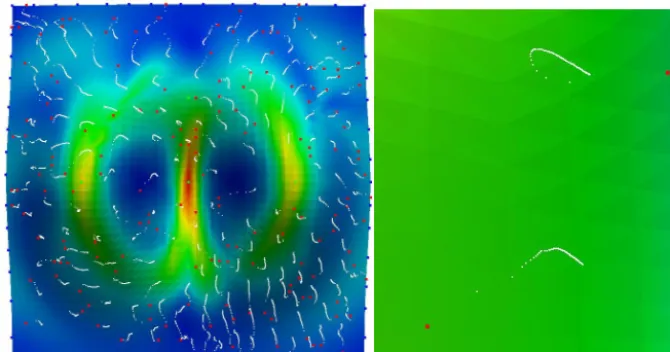
Figure 1.High-resolution grid of a mountain (Eq. 5). Left: original grid oriPd in 49×49 resolution, rendered in mean curvature. The sample points were also rendered on oirPd; the blue points are boundary points, the green points are critical points, and the red points are random points. Right: robust mean-curvature estimation. The saddle terrain features, peaks, and pits can be distinguished, compared to the depiction on the left.
Figure 2.Initial TIN surface (left) and its dual grid TD (right). The initial sample points on the dual grid are also rendered.
2.3.3 Improved CVT implementation from approximation
Lloyd’s relaxation demonstrates an effective way for heuris-tic approximation. To follow this elegant approximation, an edge bi-sectioning-based dual operation (Du et al., 2010) ap-proach is utilised. Specifically, from the sample points, an initial TIN surface is constructed. We compute its dual mesh and take this space tessellation as approximated Voronoi cells. The approximated Voronoi tessellation is then opti-mised within the cCVT iteration. But different to clustering approach, we use each approximated Voronoi cell to (verti-cally) clip the original dense DEM surface, called referring patch. From this exactly clipped referring patch, we com-pute accurate energy estimations for the new sites. The global clipping computation is localised using akd-treestructure.
The localisation and accurate referring energy computa-tion makes the cCVT iteracomputa-tion converge fast. The efficiency of the cCVT approximation as a whole is comparable to that of the elegant clustering approach (also haskd-treefast loca-tion embedded). We go no further with the complexity analy-sis, but provide an implementation of the classical clustering algorithm with the same settings as the cCVT method in the attachment. The pseudo-code of this improved cCVT itera-tion is described as follows.
Here, we illustrate this algorithm using a numerical moun-tain model. The analytic equation is
z=(4x2+y2)·e−x2−y2. (5) It has two peaks, two saddles, and a pit. We rasterise it with a 49×49=2401 regular grid (Fig. 1, left). For effectiveness, we set the transformation scale to 0.1 (ratio=0.1); i.e. there are approximately 240 points left. The sample set includes
244 X. Duan et al.: A high-fidelity multiresolution DEM for Earth systems Algorithm 2cCVT_iteration
Input: verticesN= {vi}1k, scale-transformation ratio.
1. Construct the original DEM surface oriPd from verticesN, compute density functionρbased on robust mean-curvature estimation;
2. Extract and mark boundary pointsB, mark stationary control points, check points asC, extract and mark the feature points F;
3. Perform constrained Delaunay triangulation on point set
{B, C, F}, with boundary{B}and structural terrain features
{C}as constraints; obtain an initial approximated TIN sur-face;
4. While (1E >Threshold)
{
4.1. Compute TIN’s dual TD;
4.2. For the n verticesrj in TD, extract its direct incident facets as FS= {Ti}1n;
4.3. For eachTj in FS {
4.3.1. Compute its minimal bounding box BBoxj, quickly compute its intersection with oriPd using akd-tree, ob-tain a narrowed reference geometry narrPd;
4.3.2. Compute exact intersection ofTj and narrPd, push the result into reference sets REF= {refj};
}
4.4. For each refjin REF {
4.4.1. Compute approximated Voronoi barycen-tre: x=
P
ρ·x·area(refj)
P
ρ·area(refj) ; y=
P
ρ·y·area(refj)
P
ρ·area(refj) ;
z=
P
ρ·z·area(refj)
P
ρ·area(refj) ;
4.4.2. Usekt-treefor fast intersection computation of point (x, y, z)and oriPd, with the result used as the projected nearest point; push it into the new candidate point set F0;
}
4.5. Using{B, C}as constraints, Delaunay triangulate point set{B, C, F0}and obtain reconstructed TIN0;
4.6. ComputeEon TIN0;
}
56 boundary points, 5 critical points, and an additional 169 random points for visual saturation purposes (Fig. 1, left; the red points are randomly generated points, the blue points are boundary points, and the green points are critical points). Relief feature points are always abundant in a real terrain dataset, so additional random points are rarely needed. A ro-bust mean-curvature estimation is computed on the original high-resolution surface oriPd (Fig. 1, right), from which we can clearly distinguish critical points as peaks, saddles, and pits. The initially approximated TIN surface from the sample set is shown in Fig. 2 (left), and its generated dual mesh is shown in Fig. 2 (right), which corresponds to step 3 of Al-gorithm 2. Figure 3 shows the dual cell of the sample points, which is the key idea of the cCVT approximation. Figures 4 and 5 show the algorithm steps 4.3.1 and 4.3.2, respectively,
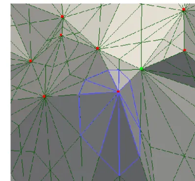
Figure 3.The triangles incident towards the first vertexri on the dual grid comprise an initial approximated Voronoi cell (rendered as a blue wireframe); the centre vertex is rendered in red.
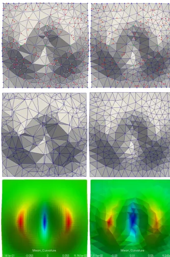
where the exact clipping is completed on the original DEM surface. Figures 6 and 7 show the final computation on the reference patch of the first sample point, which corresponds to the algorithm steps 4.4.1 and 4.4.2. Figure 8 exhibits the result of the first iteration, compared to that of the final itera-tion, with the initial sample points included (top). A compar-ison of the constructed approximate TIN grids of the initial state and final state is illustrated in the middle, while the cur-vature distribution that represents the terrain feature compar-ison is illustrated at the bottom.
The results show how the embedded stationary points (control points and boundary points), feature points, and ran-dom points are spatially equalised (Fig. 8). Additionally, the cCVT generated a variable-resolution terrain grid (middle right), the convergent TIN grid exhibited nearly uniform high quality, and the convergence process generally resembled Lloyd’s relaxation (Fig. 9).
Notably, the direct reference on the original DEM surface is realised by the exact geometry clipping, which linearly interpolated the high-resolution surface. This clipping tech-nique has several important benefits; it guarantees accurate energy estimation, it avoids the generation of invalid cluster-ing cells or zigzaggcluster-ing cells, and it promises exact site posi-tion calculaposi-tion, which will result in improved grid quality.
3 Multiresolution DEM experiments 3.1 Experimental datasets
Two sites with significant geomorphological characteristics were selected. Experimental site 1 is Mount St. Helens, lo-cated in Skamania County, WA, USA. This mountain is an active volcano, whose last eruption occurred in May 1980,
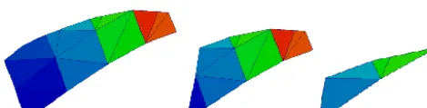
Figure 4.A triangleTj(rendered in semi-transparent blue) with its minimal bounding box’s intersection part narrPd with the original grid on the approximate grid (left), the localised intersection part narrPd (middle), and the intersection part on the original grid oriPd (right).
Figure 5.Exact clipping steps of narrPd withTi. The sequence from left to right illustrates the edge clipped results.
Figure 6.Reference patch refj on the original DEM surface of an initial Voronoi cell, with the centre atri (left). refj on the original DEM surface oriPd (right).
and deep magma chambers have been observed recently (Hand, 2015). This site was selected for its typical mountain morphology along cone ridges and evident fluvial features downhill, where heavy pyroclastic materials and deposits are present. These two distinctively different terrain structures mingle together, posing challenges for DEM generalisation.
The St. Helens dataset was selected from the Puget Sound lidar dataset (http://wagda.lib.washington.edu/data/ type/elevation/lidar/st_helens/). This lidar dataset was col-lected in late 2002. The secol-lected dataset is a 2924×3894 regular grid with a 3 m cell size and covers an area of ap-proximately 102 km2. The elevation ranges from 855.32 to 2539.34 m. The image and hillshade views of these data are illustrated in Fig. 10.
Figure 7. Barycentre computation based on the reference patch refj; the original site is the white block in the circle, and the pro-jection on oriPd of the newly computed site is depicted as the blue block in the circle.
Experimental site 2 is the Columbia Plateau, USA. This area has been labelled Universal Transverse Mercator (UTM) zone 11, so we hereafter call it UTM11 (http://gis.ess. washington.edu/data/raster/tenmeter/). This lidar dataset was collected in 2009. The selected site is located on the bor-der between Columbia County and Walla Walla County, WA. The southeastern corner is located in the Wenaha–Tucannon Wilderness, Umatilla National Forest. This area contains rugged basaltic ridges with steep canyon slopes at high eleva-tions (average of 1700 m). The northwestern area is located
246 X. Duan et al.: A high-fidelity multiresolution DEM for Earth systems
Figure 8.Comparison of converged results. Top left: reconstructed TIN surface from one iteration, with the initial points presented. Top right: the converged TIN surface with the initial sites, after approximately 140 loops. Middle: the initial approximated TIN surface (left) and the final TIN surface (right). Bottom: curvature distribution on the original surface (left) and the generalised grid (right).
near Dayton City, which is a vast agricultural and ranching area with relatively smoother morphology at low elevations (average of 500 m). This site is selected due to the coexis-tence of these two different prominent surface morphologies. If the generalisation scheme emphasises the high-elevation areas with sharp variations, the surface interpolation as a
whole might be unbalanced, which may result in smoothing of the low-elevation areas.
The selected UTM11 dataset is a 3875×3758 grid with a 10 m cell size and covers an area of over 1456 km2. The el-evation ranges from 3533 to 19 340 cm. The image and hill-shade views of these data are shown in Fig. 11.
Figure 9.Trajectories of point convergences. The red points indicate the initial sample set, and the trajectories show the convergence trends, with closer gaps between candidate points. The right side shows a close view of the convergence of two points. These trends imply that the cCVT’s convergence complies with Lloyd’s relaxation linear convergence.
Figure 10.Experimental site 1: Mount St. Helens. Left: image view. Middle: hillshade view. It is a 2924×3894 grid with a 3 m cell size.
3.2 Comparison method
As previously mentioned, DEM generalisation has long been studied in geoscience, and numerous methods have been pro-posed over time. One of the most classical approaches is the hierarchical insertion (or decimation) of feature points to construct a TIN grid under a destination scale. This type of heuristic feature point refinement (HFPR) performs very well in terms of surface approximation and terrain structure retention. For this reason, although HFPR methods generally cannot guarantee high-quality grids, these methods are suit-able for comparison purposes.
A typical HFPR starts with four corner points from a dense DEM image and constructs a Delaunay triangular grid that contains two triangles. The rest of the points are weighted
ac-cording to their distances from the triangular surface or other error criteria and then queued. The point with the highest pri-ority in the queue is selected, and the grid is modified us-ing incremental Delaunay triangulation. This process repeats until some error threshold is satisfied (Heckbert and Gar-land, 1997). Michael Garland provided a classical HFPR im-plementation (http://mgarland.org/software.html), and many other variants are available in geographic information system (GIS), meshing, and visualisation tool suites.
3.3 Quantitative comparisons
We performed the processes from Algorithm 2 for the two experimental datasets, including triangulation and curvature estimation, boundary point extraction and marking, feature
248 X. Duan et al.: A high-fidelity multiresolution DEM for Earth systems
Figure 11.Experimental site 2: UTM11 Zone. Left: image view. Middle: hillshade view. It is a 3875×3758 grid with a 10 m cell size.
Table 1.Quantitative comparison of the grid quality at scale-transformation ratio 1 %.
Dataset Dense DEM Random inter- Approx. Mean Max RMSE Max aspect points polation points method error (m) error (m) (m) ratio
St. Helen 3 m 11 386 056 230 909 cCVT 0.0353 23.05 1.6145 3.23
HFPR 0.1107 191.31 2.3714 9255
UTM11 10 m 14 562 250 301 255 cCVT 0.5773 37.70 3.77313 4.09
HFPR 0.8765 487.81 6.71214 8426
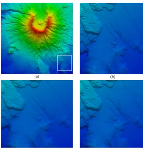
Table 2. Interpolated elevation RMSEs (m) at varied scale-transformation ratios.
Dataset Approx. 5 %∗ 1 % 0.5 % 0.1 % method
St. Helens 3 m cCVT 0.636 1.614 2.455 5.772 HFPR 1.028 2.371 4.006 11.779
UTM11 10 m cCVT 1.239 3.773 6.593 19.997 HFPR 3.087 6.712 10.137 28.460
∗The ratio percent number meansn% points left.
point extraction based on curvature significance and mark-ing, and optimisation loop through cCVT. For effectiveness, the transformation ratio was set to range from 5 to 0.1 % point density (comparable to the 3.1 to 0.6 % setting in Zhou and Chen, 2011).
The accuracy of the surface approximation determines the final surface interpolation precision and is thus a basic qual-ity comparison index. Here, we applied a statistical interpola-tion method to measure the surface approximainterpola-tion precision. From each triangle on the cCVT-generated quasi-uniform TIN grid, a random point is selected and a vertical line is introduced to intersect the original dense DEM surface and the HFPR-generalised TIN at the same time. Error estimates for the surface approximation could be obtained from these intersection points. We computed the mean error, maximum error, and root mean squared error (RMSE) for this
eleva-tion interpolaeleva-tion (TIN interpolaeleva-tion); the results are listed in Table 1. Furthermore, we computed the aspect ratios of the triangles for both generalised TIN surfaces to measure the grid quality, which are also listed in Table 1. RMSEs with various transformation ratios are listed in independent rows and columns in Table 2.
From the results in Table 1, we can conclude that under the same resolution (point density), the transformed DEM sur-face obtained using the cCVT method is generally more pre-cise than that obtained using the HFPR method. In all cases, surface approximation precision (compared to the original) decreased as the resolution coarsened.
3.4 Qualitative comparison
A qualitative index is usually measured from the aspect of terrain structure retention. According to the resulting TINs from the two experimental datasets, both the cCVT and HFPR methods performed well based on visual examination. However, upon closer inspection, the surface generated by cCVT has a smoother transition effect than that generated by HFPR (Fig. 12). HFPR accumulated more samples around sharp features (see Fig. 13), and its surface exhibited clearer impressions because flat details were smoothed out. From vi-sual examination, it may be concluded that under the same transformation conditions, HFPRs may exert a stronger gen-eralisation effect than cCVTs.
However, a stronger generalisation effect actually de-creases the precision of the general approximation, which
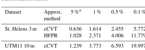
Figure 12.Visual examination of St. Helens. Top: cCVT grid. Bot-tom: HFPR grid. The latter grid appears more rigid than the former, which implies a stronger generalisation effect.
may result in structural distortion or misconfiguration. Fig-ure 14 illustrates a closer examination of St. Helens. Some structural details on the original surface were recovered by the cCVTs but not by the HFPRs. This terrain structure loss occurred on both smooth areas and steep areas, as illustrated in Fig. 14. Figure 15 illustrates similar structural detail losses by the HFPRs in the UTM11 dataset.
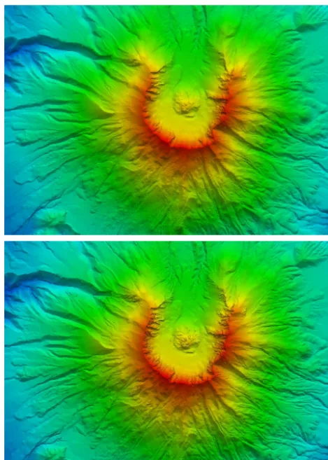
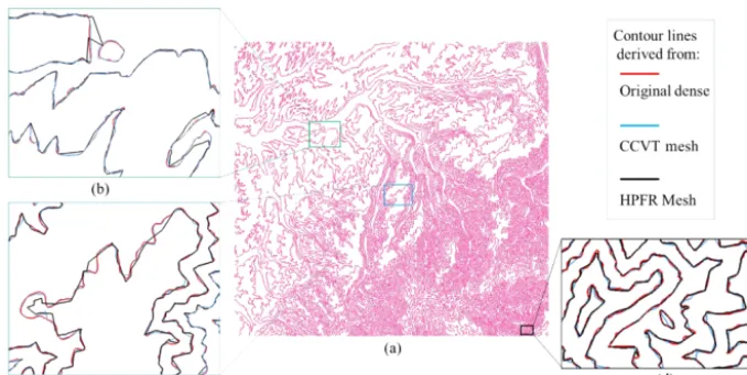
Terrain structural features could also be measured from DEM derivatives such as the slope, aspect, and hydrologi-cal structural lines. Here, we used contours to compare the generalisation accuracy using experimental site 2. For the same configurations (80 m elevation increments), we gener-ated contours for the original dense TIN (rendered in red), the cCVT-generated TIN (rendered in blue), and the HFPR-generated TIN (rendered in black), and overlaid the three sets of contours for comparison (Fig. 16). The illustrations demonstrate that in most cases (Fig. 16b, c), the contours from the cCVT-generalised surface accurately conform with those from the original dense surface, whereas the contours from the HFPR-generalised surface generally did not, except for some cases in steeper areas with sharp curvature varia-tions (Fig. 16d). This result can be explained by the HFPR’s
Figure 13.Grid quality from an intuitive comparison. Top: cCVT-generalised grid with nearly uniform triangles. Bottom: HFPR-generalised grid with irregular triangles.
stronger accumulation of sample points near sharp features, which guaranteed an edging out, if we noticed that the in-spection area (Fig. 16d) is much smaller than in panel b or c.
4 Discussion
Topography transformation of DEM surfaces has been a deeply studied topic in geoscience, simplification tech-niques and generalisation principles are widely realised and adopted. Extracting terrain feature points and using these points to construct a generalised surface has proven to be one valuable approach; its success may be due to the fea-ture points’ strong capability to capfea-ture terrain strucfea-tures. However, discrete surfaces as TIN grids that are constructed purely from feature points may not be best approximated to the original high-resolution surfaces. Take the mountain equation in Fig. 1 as an example. It has at least two peaks, two saddles, and one pit close to the zero level. Assume that the scale transformation requires that only two critical points are left; selecting both peak points is more reasonable than se-lecting the pit point, even if the pit point has a stronger
250 X. Duan et al.: A high-fidelity multiresolution DEM for Earth systems
Figure 14. Detail loss of the HFPR generalisation grid. The in-spected area in the experimental site is bounded by the white rectan-gle(a); the magnified inspection area on the original dense TIN(b); the area on the cCVT-generalised TIN (c); and the area on the HFPR-generalised TIN(d). From the close-up view, it can be seen that the HFPR method generates a rougher grid than the CVTs. Thus, structural distortion or misconfiguration might be introduced.
titative index (curvature in this case) than the peak points. This observation implies that if global surface interpolation precision is more importantly demanded, a robust approach that has overall considerations on surface approximation and terrain feature retention should be adopted.
Among those classical DEM generalisation approaches, heuristic feature point refinement is an outstanding example. As illustrated by Table 1, Figs. 12, and 16, HFPR methods perform excellently in terms of surface approximation and surface morphology retention. For the treatment of feature points, these methods use a heuristic strategy by incremental Delaunay triangulation, which considers the point with the largest error with respect to the constructed TIN. However, the impact of the insertion of a new feature point on the in-serted feature points is not considered due to computational burden. Specifically, modifications are only taking place on the triangle where the point with the largest vertical error is located. As a result, feature points may cluster around re-liefs with sharp variations, as shown in Fig. 12. Too many feature points accumulating near sharp features means that relatively few feature points are present in flat areas, which will eventually lead to terrain structure misconfiguration, as shown in Figs. 14–16. Sometimes, this type of structural loss is unacceptable. For example, the terrain relief at high ele-vation under the studied scale (10 m cell spacing) in
Figure 15. Detail loss from the HFPR method in the UTM11 dataset. The inspection area in the entire experimental site(a). The magnified view of the inspection area is shown on the original dense DEM(b), on the cCVT-generalised TIN(c), and on the HFPR-generated TIN surface(d). The fold morphology in the white ellipse was recovered by the cCVT method but not by the HFPR method.
mental site 2 exhibited a fiercer landform than at lower eleva-tions. The accumulation of too many sample points in high-elevation areas may result in the distortion of the smooth an-thropogenic terrain morphology in low-elevation areas.
cCVT starts by constructing a terrain-adaptive variable-resolution grid. The cCVT iteration uses a robust mean cur-vature as density function, which is based on the curcur-vature’s capability to characterise shapes and conduct shape evolu-tion. Under the curvature guidance, the two-step optimisation (see Algorithm 1 in Sect. 2.2) loops both to spatial equal-isation and frequency equalequal-isation. The process of spatial equalising of feature points has been seldom considered by classical approaches, which may explain why cCVT gener-ally prevails over HFPRs (see Table 1). Notably, the triangles from the spatial equalisation exhibited a maximum aspect ra-tio that was less than 5.0, which implies that the constructed terrain grid satisfied the numerical stability requirement from classical finite element or finite volume computations.
On the other hand, CVT is an approach within varia-tional framework. The result of the iteration depends on the boundary conditions and initial conditions. Hence, this ar-ticle employed a feature point scheme (with additional in-put points considered) as a relatively stationary initial con-dition to maintain algorithm stability. The requirement of embedding feature points of interest, along with consider-ation of avoiding the problematic k-means like clustering,
Figure 16.Comparison of the derived contour lines. The contours from the dense UTM11 dataset are shown in(a)and rendered in red. Three areas in the boxes were magnified to show the differences in the contour configurations. The blue contour lines are from the cCVT-generalised TIN surface, and the black lines are from the HFPR-generated TIN surface. According to the illustrations in(a)and(b), the contours that were derived from the cCVT grid (rendered in blue) are more in line with those from the original dense surface (rendered in red). The contours from the HFPR grid (rendered in black) may sometimes edge out on areas with steep slopes, as shown in(d), because the HFPR method accumulated a relatively abundant of sample points around these areas.
prompted us to develop a non-clustering approach with an exact energy referring method. Experiments on 10 million DEM points demonstrated that the exact clipping approach performed comparably to the elegant clustering approach.
5 Conclusions
In this article, a high-fidelity multiresolution DEM was proposed. The variable-resolution with high-fidelity was achieved by the developed curvature-based CVT. cCVT op-timisation increases the precision of surface approximation compared to existing heuristic DEM generalisations, while the equalisation of feature points from the spatial domain guarantees a high-quality grid.
Multiresolution models are essential tools to incorporate more scales, while a high-fidelity generalised DEM can be used to construct a concrete topographic layer from which fine endogenous or exogenous processes can be assessed un-der proper scale conditions. Evaluation of the cCVT mul-tiresolution DEM on Earth and environmental systems over wide-ranged domains and scales is a topic for future studies. Furthermore, considering the topography over a wider range may require re-implementing cCVT on the geographical ordinate base instead of on the currently used projection co-ordinate base.
6 Code and data availability
We implement the cCVT and the comparing classical k-means clustering CVT algorithm using c++ on the open-source Visualisation Toolkit (VTK; https://www.vtk.org). The approximated dual operation through edge bi-sectioning is based on the implementation of Valette et al. (2008). If anyone is interested in the technical details of the implemen-tation, please contact the corresponding author for the source codes, demo datasets, and necessary guide for compilation.
The Supplement related to this article is available online at doi:10.5194/gmd-10-239-2017-supplement.
Acknowledgement. This study is funded by the Special Fund for
Surveying, Mapping, and Geo-information Scientific Research in the Public Interest (201412014), the National Natural Science Fund of China (41271453), and Scientific and Technological Leading Talent Fund of National Administration of Surveying, Mapping, and Geo-information (2014).
Edited by: J. Neal
Reviewed by: two anonymous referees
252 X. Duan et al.: A high-fidelity multiresolution DEM for Earth systems References
Aguilar, F. J., Agüera, F., Aguilar, M. A., and Carvajal, F.: Effects of Terrain Morphology, Sampling Density, and Interpolation Meth-ods on Grid DEM Accuracy, Photogramm. Eng. Rem. S., 71, 805–816, doi:10.14358/PERS.71.7.805, 2005.
Ai, T. and Li, J.: A DEM generalization by minor valley branch detection and grid filling, ISPRS J. Photogramm., 65, 198–207, doi:10.1016/j.isprsjprs.2009.11.001, 2010.
Banchoff, T.: Critical points and curvature for embedded polyhedra, J. Differ. Geom., 77, 475–485, doi:10.2307/2317380, 1967. Bates, P. D.: Integrating remote sensing data with flood inundation
models: how far have we got?, Hydrol. Proc., 26, 2515–2521, doi:10.1002/hyp.9374, 2012.
Bilskie, M. V. and Hagen, S. C.: Topographic accuracy assessment of bare earth lidar-derived unstructured meshes, Adv. Water Re-sour., 52, 165–177, doi:10.1016/j.advwatres.2012.09.003, 2013. Bilskie, M. V., Coggin, D., Hagen, S. C., and Medeiros, S. C.: Terrain-driven unstructured mesh development through semi-automatic vertical feature extraction, Adv. Water Resour., 86, 102–118, doi:10.1016/j.advwatres.2015.09.020, 2015.
Brioude, J., Angevine, W. M., McKeen, S. A., and Hsie, E.-Y.: Numerical uncertainty at mesoscale in a Lagrangian model in complex terrain, Geosci. Model Dev., 5, 1127–1136, doi:10.5194/gmd-5-1127-2012, 2012.
Budd, C. J., Russell, R. D., and Walsh, E.: The geometry of r-adaptive meshes generated using optimal transport methods, J. Comput. Phys., 282, 113–137, doi:10.1016/j.jcp.2014.11.007, 2015.
Cabello, S., Fort, M., and Sellarès, J. A.: Higher-order Voronoi dia-grams on triangulated surfaces, Inform. Process. Lett., 109, 440– 445, doi:10.1016/j.ipl.2009.01.001, 2009.
Cea, L. and Bladé, E.: A simple and efficient unstructured fi-nite volume scheme for solving the shallow water equations in overland flow applications, Water Resour. Res., 51, 5464–5486, doi:10.1002/2014WR016547, 2015.
Chen, C. and Li, Y.: An orthogonal least-square-based method for DEM generalization, Int. J. Geogr. Inf. Sci., 27, 154–167, doi:10.1080/13658816.2012.674136, 2012.
Chen, C., Li, Y., and Yue, T.: Surface modeling of DEMs based on a sequential adjustment method, Int. J. Geogr. Inf. Sci., 27, 1272– 1291, doi:10.1080/13658816.2012.704037, 2012.
Chen, C., Yan, C., Cao, X., Guo, J., and Dai, H.: A greedy-based multiquadric method for LiDAR-derived ground data reduction, ISPRS J. Photogramm., 102, 110–121, doi:10.1016/j.isprsjprs.2015.01.012, 2015.
Chen, Y. and Zhou, Q.: A scale-adaptive DEM for multi-scale terrain analysis, Int. J. Geogr. Inf. Sci., 27, 1329–1348, doi:10.1080/13658816.2012.739690, 2012.
Cohen-Steiner, D., Alliez, P., and Desbrun, M.: Variational shape approximation, ACM Trans. Graph., 23, 905–914, doi:10.1145/1186562.1015817, 2004.
Du, Q., Faber, V., and Gunzburger, M.: Centroidal Voronoi Tessella-tions: Applications and Algorithms, SIAM Review, 41, 637–676, doi:10.1137/S0036144599352836, 1999.
Du, Q., Gunzburger, M. D., and Ju, L.: Constrained Centroidal Voronoi Tessellations for Surfaces, SIAM J. Sci. Comput., 24, 1488–1506, doi:10.1137/S1064827501391576, 2003.
Du, Q., Max, G., and Ju, L.: Advances in Studies and Applications of Centroidal Voronoi Tessellations, Numer. Math. Theor. Meth. Appl., 3, 119–142, doi:10.4208/nmtma.2010.32s.1, 2010. Fiddes, J. and Gruber, S.: TopoSCALE v.1.0: downscaling gridded
climate data in complex terrain, Geosci. Model Dev., 7, 387–405, doi:10.5194/gmd-7-387-2014, 2014.
Florinsky, I. and Pankratov, A.: Digital terrain modeling with the Chebyshev polynomials, arXiv preprint arXiv:1507.03960, 2015.
Glover, R. W.: Influence of Spatial Resolution and Treatment of Orography on GCM Estimates of the Surface Mass Bal-ance of the Greenland Ice Sheet, J. Climate, 12, 551–563, doi:10.1175/1520-0442(1999)012<0551:IOSRAT>2.0.CO;2, 1999.
Guba, O., Taylor, M. A., Ullrich, P. A., Overfelt, J. R., and Levy, M. N.: The spectral element method (SEM) on variable-resolution grids: evaluating grid sensitivity and resolution-aware numerical viscosity, Geosci. Model Dev., 7, 2803–2816, doi:10.5194/gmd-7-2803-2014, 2014.
Guilbert, E., Gaffuri, J., and Jenny, B.: Terrain Generalisation, in: Abstracting Geographic Information in a Data Rich World, edited by: Burghardt, D., Duchêne, C., and Mackaness, W., Lec-ture Notes in Geoinformation and Cartography, Springer Interna-tional Publishing, 2014.
Hand, E.: Deep magma chambers seen beneath Mount St. Helens, available at http://www.sciencemag.org/news/2015/11/ deep-magma-chambers-seen-beneath-mount-st-helens, 2015. Heckbert, P. S. and Garland, M.: Survey of polygonal surface
sim-plification algorithms, DTIC Document, 1997.
Hughes, J. K., Ross, A. N., Vosper, S. B., Lock, A. P., and Jemmett-Smith, B. C.: Assessment of valley cold pools and clouds in a very high-resolution numerical weather prediction model, Geosci. Model Dev., 8, 3105–3117, doi:10.5194/gmd-8-3105-2015, 2015.
Hunter, N. M., Bates, P. D., Horritt, M. S., and Wilson, M. D.: Simple spatially-distributed models for predicting flood inundation: A review, Geomorphology, 90, 208–225, doi:10.1016/j.geomorph.2006.10.021, 2007.
Jenny, B., Jenny, H., and Hurni, L.: Terrain Generalization with Multi-scale Pyramids Constrained by Curvature, Cartogr. Geogr. Inform., 38, 110–116, doi:10.1559/15230406382110, 2011. Jiménez, P. A. and Dudhia, J.: On the Ability of the WRF Model to
Reproduce the Surface Wind Direction over Complex Terrain, J. Appl. Meteorol. Climatol., 52, 1610–1617, doi:10.1175/JAMC-D-12-0266.1, 2013.
Ke, Y., Leung, L. R., Huang, M., Coleman, A. M., Li, H., and Wig-mosta, M. S.: Development of high resolution land surface pa-rameters for the Community Land Model, Geosci. Model Dev., 5, 1341–1362, doi:10.5194/gmd-5-1341-2012, 2012.
Kennelly, P. J.: Terrain maps displaying hill-shading with curvature, Geomorphology, 102, 567–577, doi:10.1016/j.geomorph.2008.05.046, 2008.
Kesserwani, G. and Liang, Q.: Dynamically adaptive grid based dis-continuous Galerkin shallow water model, Adv. Water Resour., 37, 23–39, doi:10.1016/j.advwatres.2011.11.006, 2012. Kim, B., Sanders, B. F., Schubert, J. E., and Famiglietti, J. S.: Mesh
type tradeoffs in 2D hydrodynamic modeling of flooding with a Godunov-based flow solver, Adv. Water Resour., 68, 42–61, doi:10.1016/j.advwatres.2014.02.013, 2014.
Kimmel, R. and Sethian, J. A.: Computing geodesic paths on mani-folds, P. Natl. Acad. Sci. USA, 95, 8431–8435, 1998.
Kumar, S. V., Peters-Lidard, C. D., Santanello, J., Harrison, K., Liu, Y., and Shaw, M.: Land surface Verification Toolkit (LVT) – a generalized framework for land surface model evaluation, Geosci. Model Dev., 5, 869–886, doi:10.5194/gmd-5-869-2012, 2012.
Lee, J. A. Y.: Comparison of existing methods for building tri-angular irregular network, models of terrain from grid dig-ital elevation models, Int. J. Geogr. Inf. Syst., 5, 267–285, doi:10.1080/02693799108927855, 1991.
Leempoel, K., Parisod, C., Geiser, C., Daprà, L., Vittoz, P., and Joost, S.: Very high-resolution digital elevation models: are multi-scale derived variables ecologically relevant?, Method. Ecol. Evol., 6, 1373–1383, doi:10.1111/2041-210X.12427, 2015.
Lloyd, S.: Least squares quantization in PCM, IEEE T. Inform. The-ory, 28, 129–137, doi:10.1109/TIT.1982.1056489, 1982. Meyer, M., Desbrun, M., Schröder, P., and Barr, A.: Discrete
Differential-Geometry Operators for Triangulated 2-Manifolds, in: Visualization and Mathematics III, edited by: Hege, H.-C. and Polthier, K., Mathematics and Visualization, Springer Berlin Heidelberg, doi:10.1007/978-3-662-05105-4_2, 2003.
Milnor, J. W.: Morse theory, Princeton university press, 1963. Mitášová, H. and Hofierka, J.: Interpolation by regularized
spline with tension: II. Application to terrain modeling and surface geometry analysis, Math. Geol., 25, 657–669, doi:10.1007/BF00893172, 1993.
Nikolos, I. K. and Delis, A. I.: An unstructured node-centered finite volume scheme for shallow water flows with wet/dry fronts over complex topography, Comput. Method. Appl. M, 198, 3723– 3750, doi:10.1016/j.cma.2009.08.006, 2009.
Nunalee, C. G., Horváth, Á., and Basu, S.: High-resolution nu-merical modeling of mesoscale island wakes and sensitivity to static topographic relief data, Geosci. Model Dev., 8, 2645–2653, doi:10.5194/gmd-8-2645-2015, 2015.
Pan, H., Choi, Y.-K., Liu, Y., Hu, W., Du, Q., Polthier, K., Zhang, C., and Wang, W.: Robust modeling of constant mean curvature surfaces, ACM Trans. Graph., 31, 1–11, doi:10.1145/2185520.2185581, 2012.
Ringler, T., Ju, L., and Gunzburger, M.: A multiresolution method for climate system modeling: application of spherical cen-troidal Voronoi tessellations, Ocean Dynam., 58, 475–498, doi:10.1007/s10236-008-0157-2, 2008.
Ringler, T. D., Jacobsen, D., Gunzburger, M., Ju, L., Duda, M., and Skamarock, W.: Exploring a Multiresolution Modeling Ap-proach within the Shallow-Water Equations, Mon. Weather Rev., 139, 3348–3368, doi:10.1175/MWR-D-10-05049.1, 2011.
Schneider, B.: Extraction of Hierarchical Surface Networks from Bilinear Surface Patches, Geogr. Anal., 37, 244–263, doi:10.1111/j.1538-4632.2005.00638.x, 2005.
Shi, W. Z., Li, Q. Q., and Zhu, C. Q.: Estimating the propagation error of DEM from higher-order interpola-tion algorithms, Int. J. Remote Sens., 26, 3069–3084, doi:10.1080/01431160500057905, 2005.
Tarolli, P.: High-resolution topography for understanding Earth sur-face processes: Opportunities and challenges, Geomorphology, 216, 295–312, doi:10.1016/j.geomorph.2014.03.008, 2014. Valette, S. and Chassery, J.-M.: Approximated Centroidal
Voronoi Diagrams for Uniform Polygonal Mesh Coarsen-ing, Comput. Graph. Forum, 23, 381–389, doi:10.1111/j.1467-8659.2004.00769.x, 2004.
Valette, S., Chassery, J. M., and Prost, R.: Generic Remesh-ing of 3D Triangular Meshes with Metric-Dependent Discrete Voronoi Diagrams, IEEE T. Vis. Comput. Gr., 14, 369–381, doi:10.1109/TVCG.2007.70430, 2008.
Weibel, R.: Models and Experiments for Adaptive Computer-Assisted Terrain Generalization, Cartogr. Geogr. Inform., 19, 133–153, doi:10.1559/152304092783762317, 1992.
Weller, H., Weller, H. G., and Fournier, A.: Voronoi, Delaunay, and Block-Structured Mesh Refinement for Solution of the Shallow-Water Equations on the Sphere, Mon. Weather Rev., 137, 4208– 4224, doi:10.1175/2009MWR2917.1, 2009.
Weller, H., Browne, P., Budd, C., and Cullen, M.: Mesh adaptation on the sphere using optimal transport and the numerical solution of a Monge–Ampère type equation, J. Comput. Phys., 308, 102– 123, doi:10.1016/j.jcp.2015.12.018, 2016.
Wilby, R. L. and Wigley, T. M. L.: Downscaling general circulation model output: a review of methods and limitations, Prog. Phys. Geog., 21, 530–548, doi:10.1177/030913339702100403, 1997. Wilson, J. P.: Digital terrain modeling, Geomorphology, 137, 107–
121, doi:10.1016/j.geomorph.2011.03.012, 2012.
Wilson, J. P. and Gallant, J. C.: Terrain Analysis: Principles and Ap-plications, in: Digital Terrain Analysis, Wiley, New York, 2000. Zakšek, K. and Podobnikar, T.: An effective DEM generalization
with basic GIS operations, 8th ICA WORKSHOP on Generali-sation and Multiple Representation, A Coru´na, Spain, 7–8 July, 2005.
Zarzycki, C. M., Jablonowski, C., and Taylor, M. A.: Using Variable-Resolution Meshes to Model Tropical Cyclones in the Community Atmosphere Model, Mon. Weather Review, 142, 1221–1239, doi:10.1175/MWR-D-13-00179.1, 2014.
Zhou, Q. and Chen, Y.: Generalization of DEM for terrain analysis using a compound method, ISPRS J. Photogramm., 66, 38–45, doi:10.1016/j.isprsjprs.2010.08.005, 2011.