The SOCOL version 3.0 chemistry–climate model: description, evaluation, and implications from an advanced transport algorithm

(1)

Geosci. Model Dev., 6, 1407–1427, 2013 www.geosci-model-dev.net/6/1407/2013/ doi:10.5194/gmd-6-1407-2013

EGU Journal Logos (RGB)

Advances in

Geosciences

Open Access

Natural Hazards

and Earth System

Sciences

Open Access

Annales

Geophysicae

Open Access

Nonlinear Processes

in Geophysics

Open Access

Atmospheric

Chemistry

and Physics

Open Access

Atmospheric

Chemistry

and Physics

Open Access Discussions

Atmospheric

Measurement

Techniques

Open Access

Atmospheric

Measurement

Techniques

Biogeosciences

Open Access Open Access

Biogeosciences

Discussions

Climate

of the Past

Climate

of the Past

Discussions

Earth System

Dynamics

Earth System

Dynamics

Discussions

Geoscientific

Instrumentation

Methods and

Data Systems

Open Access

_{Geoscientific}

Instrumentation

Methods and

Data Systems

Geoscientific

Model Development

Geoscientific

Model Development

Discussions

Hydrology and

Earth System

Sciences

Open Access

Hydrology and

Earth System

Sciences

Ocean Science

Discussions

Solid Earth

Discussions

The Cryosphere

Discussions

Natural Hazards

and Earth System

Sciences

Open Access

Discussions

The SOCOL version 3.0 chemistry–climate model: description,

evaluation, and implications from an advanced transport algorithm

A. Stenke1, M. Schraner1,*, E. Rozanov1,2, T. Egorova2, B. Luo1, and T. Peter1

1_{Institute for Atmospheric and Climate Science, ETH Zurich, Switzerland}

2_{Physical-Meteorological Observatory/World Radiation Center, Davos, Switzerland} *_{now at: MeteoSwiss, Zurich, Switzerland}

Correspondence to: A. Stenke ([email protected])

Received: 26 July 2012 – Published in Geosci. Model Dev. Discuss.: 30 October 2012 Revised: 20 July 2013 – Accepted: 24 July 2013 – Published: 9 September 2013

Abstract. We present the third generation of the coupled chemistry–climate model (CCM) SOCOL (modeling tools for studies of SOlar Climate Ozone Links). The most notable modifications compared to the previous model version are (1) the dynamical core has been updated with the fifth gen-eration of the middle-atmosphere general circulation model MA-ECHAM (European Centre/HAMburg climate model), and (2) the advection of the chemical species is now calcu-lated by a mass-conserving and shape-preserving flux-form transport scheme instead of the previously used hybrid ad-vection scheme. The whole chemistry code has been rewrit-ten according to the ECHAM5 infrastructure and transferred to Fortran95. In contrast to its predecessors, SOCOLvs3 is now fully parallelized. The performance of the new SOCOL version is evaluated on the basis of transient model simula-tions (1975–2004) with different horizontal (T31 and T42) resolutions, following the approach of the CCMVal-1 model validation activity. The advanced advection scheme signifi-cantly reduces the artificial loss and accumulation of tracer mass in regions with strong gradients that was observed in previous model versions. Compared to its predecessors, SOCOLvs3 generally shows more realistic distributions of chemical trace species, especially of total inorganic chlorine, in terms of the mean state, but also of the annual and interan-nual variability. Advancements with respect to model dynam-ics are for example a better representation of the stratospheric mean state in spring, especially in the Southern Hemisphere, and a slowdown of the upward propagation in the tropical lower stratosphere. Despite a large number of improvements model deficiencies still remain. Examples include a too-fast

vertical ascent and/or horizontal mixing in the tropical strato-sphere, the cold temperature bias in the lowermost polar stratosphere, and the overestimation of polar total ozone loss during Antarctic springtime.

1 Introduction

The accurate calculation of the advective transport of chem-ical species is of fundamental importance for the overall performance of coupled chemistry–climate models (CCMs). Deficiencies in the transport scheme may lead to errors in the spatial distribution and temporal evolution of ozone and other chemical trace gases that react with ozone, e.g., chlorine- and bromine-containing species (Schraner et al., 2008; Stenke et al., 2008, 2009). Furthermore, model biases in tracer dis-tributions may negatively affect model dynamics via radia-tive feedback. The increasing number of chemical species considered and complex feedback processes makes modern chemistry–climate models more and more vulnerable to lim-itations of applied numerical schemes.

(2)

1408 A. Stenke et al.: The SOCOL version 3.0 chemistry–climate model

is that the Courant–Friedrichs–Lewy (CFL) stability condi-tion (Courant et al., 1928) does not need to be fulfilled, en-abling large advection time steps (even near the poles, where the small cell sizes provoke the violation of the CFL cri-terion). In previous model versions an advection time step of two hours has been applied, making SOCOL computa-tionally very efficient. Furthermore, semi-Lagrangian meth-ods are computationally less expensive than, e.g., flux-form schemes (Rasch and Lawrence, 1998). However, this issue is becoming less critical with improvements in modern com-puter technology. The disadvantage of the semi-Lagrangian approach is the lack of mass conservation, which requires the application of so-called mass fixers after each advection time step (Williamson and Rasch, 1989) to ensure global mass conservation. The application of mass correction on the global scale, however, may lead to artificial mass transport and undesirable accumulation or loss of mass in particular regions. This problem is most dangerous in areas character-ized by sharp tracer gradients, such as the edge of the polar vortex. Erroneous concentrations can then be transported to other model layers, leading to non-physical tracer distribu-tions (Schraner et al., 2008).

In SOCOLvs1.0 the deficiencies of the semi-Lagrangian advection scheme became most apparent in the simulated distribution of total organic and inorganic chlorine (CCly1).

Since surface emissions of chlorofluorocarbons (CFCs) and tropospheric wash-out of HCl are the only source and sink processes of total chlorine in the model, CCly is expected

to behave as a passive tracer with a relatively smooth dis-tribution throughout the stratosphere and mesosphere. How-ever, the stratospheric mixing ratio of total inorganic chlorine (Cly) simulated with SOCOLvs1.0 was up to 30 % higher

than the maximum amount of total chlorine (CCly)

enter-ing the stratosphere (see Schraner et al., 2008, their Fig. 1). Moreover, unrealistic CCly minima appeared in high

lati-tudes around 50 hPa during winter and spring, most promi-nent over Antarctica, with values up to 50 % lower than any-where else. This example demonstrates the artificial mass ac-cumulation and loss caused by the semi-Lagrangian advec-tion scheme and its mass fixer routine.

Schraner et al. (2008) described a simple, efficient method to reduce these transport-related shortcomings for modeled chlorine, bromine and nitrogen species. The idea of the so-called “family-based mass correction” is based on the fact that relatively smooth tracer distributions, such as those of the Cly, Bry and NOy families, are much less critical for

transport errors than inhomogeneous distributions of indi-vidual family members. Therefore, the respective families are transported in addition to the individual family members, and the mass fixer is no longer applied to the family mem-bers, but to the transported family. The mixing ratio of the

1_{Definition of the total chlorine family within SOCOL:}

[CCly]=[Cl]+[ClO]+[HOCl]+2[Cl2]+2[Cl2O2]+[BrCl]+[HCl]

+ [ClONO2]+[Cl-atoms in ODS]

transported, mass-corrected family is then used to re-scale the mixing ratios of the family members in every grid box. This method ensures local mass conservation and led to a number of model improvements in SOCOLvs2.

As shown by Schraner et al. (2008), this simple concept, while considerably reducing the deficiencies of the semi-Lagrangian scheme, cannot fully eliminate them. Firstly, even the Cly, Bryand NOyfamilies are not completely

homo-geneous, but have strong gradients at the tropopause. There-fore the mass fixer affects the tracer families themselves. Sec-ondly, the method can only be applied to chemical species belonging to a family. For chemical species without a cor-responding family, for example ozone itself, an alternative method has to be applied as, for example, restricting the mass fixer to certain geographical regions (Schraner et al., 2008). However, compared to Clyor Bry the stratospheric lifetime

of the Oxfamily is much shorter, and, therefore, mass

conser-vation during advection becomes less critical than for tracers with a lifetime longer than one year. From all of this it is ob-vious that a more satisfying approach to the advection prob-lem requires the semi-Lagrangian scheme to be replaced by a more advanced, mass-conserving approach.

Here we present an updated version (vs3) of the COL CCM. The two most important modifications of SO-COLvs3 compared to its predecessors are (1) the underly-ing general circulation model has been updated from the middle-atmosphere GCM MA-ECHAM4 (European Cen-tre/HAMburg climate model; Roeckner et al., 1996; Manzini and Bengtsson, 1996) to MA-ECHAM5 (Roeckner et al., 2003, 2006; Manzini et al., 2006), and (2) the advection of the chemical trace species is now calculated by the flux-form semi-Lagrangian scheme of Lin and Rood (1996) in-stead of the previously applied hybrid advection scheme. The hybrid approach has been described in detail by Zubov et al. (1999). The hybrid advection scheme uses the opera-tor splitting approach; i.e., vertical and horizontal transport are calculated separately. In the vertical direction it utilizes the Eulerian scheme proposed by Prather (1986), while in the horizontal direction a semi-Lagrangian scheme (Ritchie, 1985; Williamson and Rasch, 1989) is applied. The advec-tion scheme of Lin and Rood (1996), which is operaadvec-tionally implemented in (MA-)ECHAM5, is a multidimensional flux-form scheme and by construction mass conservative to ma-chine precision. It also can cope with long time steps to make it applicable within GCMs. In addition to mass conserva-tion, the advection scheme of Lin and Rood (1996) satisfies other fundamental requirements for tracer algorithms, such as monotonicity and conservation of tracer correlations. Fur-thermore, the advection scheme very effectively prevents nu-merical diffusion.

In SOCOLvs1 and vs2, the chemistry module code was not parallelized and the model could therefore only be run on a single CPU. To take advantage of modern, parallel computer architectures the parallelization of the chemistry code was a further, important goal. For SOCOLvs3 the chemistry code

(3)

has been transferred to Fortran95 and completely redesigned according to the ECHAM5 infrastructure and modularity.

The intention of this paper is to provide a technical description of the new version SOCOLvs3 and to evalu-ate the performance of the upgraded model with respect to model dynamics and chemistry, documenting model improvements and identifying remaining deficiencies. As in previous model evaluation publications, this study is based on transient model simulations with horizontal reso-lution T31 (3.75◦×3.75◦) covering the years 1975–2004, including numerous natural and anthropogenic forcings. In addition, we here also use horizontal resolution T42 (2.8◦×2.8◦). The analysis of the model results follows the guidelines of the WCRP/SPARC (World Climate Research Programme/Stratospheric Processes and their Role in Cli-mate) chemistry–climate model validation activity CCMVal-1 (Eyring et al., 2006). The CCMVal-2 initiative (SPARC, 2010) used a more advanced and extensive set of diagnos-tics, which goes beyond the scope of this paper.

The following section provides a description of the new model version SOCOLvs3. The experimental set-up of the model simulations is briefly described in Sect. 3. Section 4 shows the effects of the replaced advection scheme using the example of the chlorine family. In Sect. 5, the new model version is evaluated against observations, focusing on strato-spheric dynamics and chemistry. Differences from the previ-ous model version SOCOLvs2 are also documented.

2 SOCOLvs3 model description

The coupled chemistry–climate model SOCOL consists of the middle-atmosphere GCM MA-ECHAM and a modified version of the chemistry-transport model (CTM) MEZON (Model for Evaluation of oZONe trends; Rozanov et al., 1999, 2001; Egorova et al., 2001, 2003; Hoyle, 2005; Schraner et al., 2008). The GCM and CTM are interac-tively coupled by the 3-dimensional fields of temperature and wind, and by the radiative forcing induced by water va-por, ozone, methane, nitrous oxide, and chlorofluorocarbons (CFCs). The CTM is called every 2 h, making SOCOL com-putationally very efficient. From a technical point of view, the coupling between GCM and CTM has been greatly sim-plified. The MEZON code has been transferred from For-tran77 to Fortran95 and completely rewritten according to the ECHAM5 infrastructure. In contrast to previous versions, the model can now be run in parallel mode. On parallel com-puting infrastructure, this enables a further reduction of the wall clock time, which has already been an attractive fea-ture of SOCOLvs1 and vs2. For comparison, one model year with SOCOLvs2 required about two days on a single CPU (Schraner et al., 2008), while SOCOLvs3 requires about 4 h for one model year (on 32 CPUs, T31 horizontal resolution, 39 vertical levels).

2.1 MA-ECHAM5

MA-ECHAM5 (Manzini et al., 2006) is the recent middle-atmosphere version of the ECHAM GCM developed at the MPI for Meteorology, Hamburg. ECHAM originally evolved from the spectral weather prediction model of the Euro-pean Centre of Medium-Range Weather Forecasts (ECMWF; Simmons et al., 1989), extended by a comprehensive parame-terization package for climate applications. A detailed model description of ECHAM5 is given by Roeckner et al. (2003, 2006). Within SOCOLvs3, the MA-ECHAM model version 5.4.00 is used.

All versions of ECHAM are spectral general circulation models based on the primitive equations with the prognos-tic variables temperature, vorprognos-ticity, divergence, logarithm of surface pressure, humidity and cloud water. Tracer transport and model physics are calculated on a Gaussian transform grid. In the vertical, a hybrid sigmap coordinate system is used. The middle-atmosphere version MA-ECHAM5 can be run with 39 or 90 vertical levels. The model top is centered at 0.01 hPa (∼80 km), for both vertical resolutions. Within SOCOLvs3, 39 levels are used by default. The model time step for dynamical processes and physical parameterizations is 15 min.

Compared to ECHAM4, several parameterizations of physical processes have been changed in ECHAM5. A new parameterization of stratiform clouds has been developed, in-cluding a separate treatment of cloud water and cloud ice, advanced cloud microphysics and a statistical model for the calculation of cloud cover. The description of coupling pro-cesses between the land surface and the atmosphere has been improved, including a new land surface dataset.

Water vapor, cloud variables and chemical species are advected by a flux-based mass-conserving and shape-preserving transport scheme (Lin and Rood, 1996), instead of the semi-Lagrangian approach used in ECHAM4. The scheme is designed for time steps of arbitrary length. Thus, as for a semi-Lagrangian scheme, the CFL stability criterion does not need to be fulfilled.

The shortwave radiation scheme is based on the radiation code of the ECMWF (Fouquart and Bonnel, 1980), and basi-cally the same as in ECHAM4. However, the spectral res-olution has been increased from 2 to 6 bands, with three bands in the UV-visible range (185–250 nm, 250–440 nm, 440–690 nm) and three bands in the near-IR range (690– 1190 nm, 1190–2380 nm, 2380–4000 nm) (Cagnazzo et al., 2007). To obtain realistic heating rates in the mesosphere, SOCOL additionally takes account of the absorption by O2

and O3in the Lyman-alpha emission line of solar hydrogen

(121.6 nm) and the O2Schumann–Runge absorption bands

(175–200 nm); see Egorova et al. (2004). This parameteriza-tion is not part of the original (MA-)ECHAM5 code.

(4)

Model) scheme (Mlawer et al., 1997), based on the more accurate k correlated method, is used. Compared to MA-ECHAM4, the number of spectral intervals has been in-creased from 6 to 16 longwave bands. Full radiative transfer calculations are performed every 2 h. The calculated long-wave fluxes are kept constant over the whole radiation time step, while the shortwave fluxes are updated each dynamical time step, accounting for changes in the local zenith angle.

The parameterization of the effects of the gravity wave spectrum is based on the so-called Doppler spread theory and follows the formulation of Hines (1997a, b). The source spec-trum of the Hines scheme is given by Manzini et al. (2006).

2.2 MEZON

The CTM MEZON has the same vertical and horizontal grid as MA-ECHAM5; i.e., the chemical calculations are per-formed on the Gaussian grid with a hybrid sigma p co-ordinate in the vertical. The model includes 41 chemical species of the oxygen, hydrogen, nitrogen, carbon, chlo-rine and bromine groups, which are determined by 140 gas-phase reactions, 46 photolysis reactions and 16 heteroge-neous reactions in/on aqueous sulfuric acid aerosols as well as three types of polar stratospheric clouds (PSCs), super-cooled ternary solution (STS) droplets, water ice and nitric acid trihydrate (NAT).

The parameterization of heterogeneous chemistry is based on Carslaw et al. (1995). It takes into account HNO3uptake

by aqueous sulfuric acid aerosols resulting in the formation of STS. The parameterization of the liquid-phase reactive up-take coefficients follows Hanson and Ravishankara (1994) and Hanson et al. (1996). The PSC scheme for water ice uses a prescribed particle number density of 0.01 cm−3

(in-stead of 0.1 cm−3used in SOCOLvs2) and assumes that the cloud particles are in thermodynamic equilibrium with their gaseous environment. NAT is formed if the partial pressure of HNO3exceeds its saturation pressure, assuming a mean

particle radius of 5 µm for NAT. The particle number den-sities are limited by an upper boundary of 5×10−4cm−3 to account for the fact that observed NAT clouds are often strongly supersaturated, which is a numerically cheap ther-modynamic approximation for the slow growth kinetics of these particles. The sedimentation of NAT and water ice is based on the Stokes theory as described in Pruppacher and Klett (1997). Water ice and NAT are not explicitly trans-ported, but are evaporated back to water vapor and gaseous HNO3after each chemical time step, transported in the

va-por phase, and then depending on the saturation conditions regenerated in the next time step with the thermodynamic approximation described above.

The chemical reaction rate coefficients are taken from Sander et al. (2006). Photolysis rates are calculated at every chemical time step using a look-up-table approach (Rozanov et al., 1999), including effects of the solar irradiance vari-ability. The impact of cloudiness on photolysis rates already

has been included in an extended tropospheric version of SO-COL, but not in the operational model, as presented here. The chemical solver is based on the implicit iterative Newton– Raphson scheme (Ozolin, 1992; Stott and Harwood, 1993). Chemical calculations are performed every 2 h.

MEZON considers dry deposition of O3, CO, NO, NO2,

HNO3 and H2O2. Dry deposition velocities over land and

sea are based on Hauglustaine et al. (1994). Furthermore, the tropospheric wash-out of HNO3 is described by a constant

removal rate of 4×10−6s−1; i.e., every two hours 2.8 % of the tropospheric HNO3is removed.

In contrast to SOCOLvs2, the transport of the chemical trace species is calculated with the advection scheme of Lin and Rood (1996) implemented in MA-ECHAM5, instead of the hybrid scheme of Zubov et al. (1999), which was part of MEZON. As in the previous model version, each individual chemical species of the Cly, Bry, and NOyfamilies are

trans-ported (as well as the families themselves in order to still be able to apply a family correction; see below). In contrast to previous model versions, the transport is calculated every dynamical time step (15 min) instead of every 2 h.

SOCOLvs2 differentiated two water vapor fields: the one of the GCM used below 100 hPa, which included the com-plete hydrological cycle in the troposphere, and the one of the CTM used above 100 hPa to account for water vapor pro-duction/destruction by chemical reactions. In vs3, this un-satisfying separation has become obsolete. SOCOLvs3 con-siders only one water vapor field, i.e., the ECHAM5 water vapor. Large-scale advection, cumulus convection and the tropospheric hydrological cycle are calculated by the GCM, while chemical water vapor production/destruction as well as PSC formation are calculated by the chemistry module. To avoid interference of the ECHAM5 cloud scheme and the PSC routine, we ensure that the ECHAM5 parameterization of stratiform clouds is deactivated in the stratosphere.

3 Model set-up and boundary conditions

The evaluation of the new model version SOCOLvs3 is based on two transient model simulations from 1975 to 2004, for T31 and T42 horizontal resolutions. Both model simulations were performed with a vertical resolution of 39 levels. The simulation set-up follows the specifications of the CCMVal-2 reference simulation REF-B1 (Eyring et al., CCMVal-2008), which was designed to reproduce past atmospheric conditions as realistically as possible. The simulations are driven by sev-eral natural and anthropogenic forcings, such as the 11 yr so-lar cycle, the quasi-biennial oscillation (QBO), stratospheric sulfate aerosol loading, as well as changes in trace gas con-centrations.

Global sea surface temperatures (SSTs) and sea ice cov-erage (SIC) are prescribed as monthly means following the HadISST1 dataset provided by the UK Met Office Hadley Centre (Rayner et al., 2003). The dataset is based on merged satellite and in situ observations.

(5)

Atmospheric concentrations of the most relevant green-house gases (CO2, CH4, N2O) for the years before 1996

are prescribed following IPCC (2001). This time series is merged with NOAA observations from 1997 to 2004 (Eyring et al., 2008). Time-dependent surface mixing ratios of ozone-depleting substances (ODS) are taken from WMO (2007). Emission fluxes of CO and nitrogen oxides (NOx) from

in-dustrial sources, traffic and biomass burning are taken from the RETRO dataset (Schultz and Rast, 2007), whereas emis-sions from soils and oceans follow Horowitz et al. (2003). For NOx emissions from aircraft the dataset described by

Dameris et al. (2005) is used. NOx emissions from

light-ning are based on the satellite-based dataset of Turman and Edgar (1982), with a global annual NOxproduction of

4 Tg(N) yr−1.

The chemical effect of the enhanced stratospheric aerosol loading after the two major volcanic eruptions of El Chich´on (1982) and Mount Pinatubo (1991) is considered by prescribing observed sulfate aerosol surface area densities (SADs) as monthly means. The SAD time series is based on SAGE I, SAGE II, SAM II and SME observations and covers the period from 1979 to 2005. More details about the merged SAD time series are given in Eyring et al. (2008). The ra-diative effects of volcanic eruptions are calculated online. For this purpose the extinction coefficient, asymmetry fac-tor, and single scattering albedo of the stratospheric aerosol record were pre-calculated using Mie theory as described in Schraner et al. (2008), with the aerosol surface area den-sity and the effective aerosol radius (both obtained from the SAGE dataset by Thomason and Peter, 2006) as input pa-rameters. A tropospheric aerosol climatology (Lohmann et al., 1999) is used for the calculation of local heating rates and shortwave backscatter. Aerosol–cloud interactions and heterogeneous chemistry on tropospheric aerosols or clouds are not considered in SOCOL.

The QBO is forced by a linear relaxation (“nudging”) of the simulated zonal winds in the equatorial stratosphere to a time series of observed wind profiles (Giorgetta, 1996). The nudging is applied between 20◦N and 20◦S from 90 hPa up to 3 hPa. Within the QBO core domain (10◦N–10◦S, 50– 8 hPa) the relaxation time is uniformly set to 7 days; outside this region the damping depends on latitude and altitude. It should be mentioned that the described nudging approach is only necessary for the model version with 39 levels. The ver-sion of MA-ECHAM5 with 90 vertical levels spontaneously simulates a QBO (Giorgetta et al., 2006).

The variability of solar irradiance has been taken into ac-count for the calculations of the solar radiation fluxes, photol-ysis and heating rates, using the time series of monthly mean extra-terrestrial spectral solar irradiance (SSI) compiled by Lean et al. (2005). These data were used to calculate the in-tegrated extra-terrestrial solar fluxes for the six intervals of the MA-ECHAM5 solar radiation code, as well as the pa-rameters for the parameterization of the heating rates due to absorption at wavelengths of the Lyman-alpha line and

Schumann–Runge bands. The SSI time series was also used to calculate monthly look-up tables for the calculation of the photolysis rates in the chemical part of the model.

4 Effects of the new advection scheme

In this section, we demonstrate the effects of the new ad-vection scheme using the example of the total chlorine fam-ily (total inorganic plus organic chlorine, CCly). Except

ex-change with the troposphere, there are no further sources or sinks of total chlorine in the stratosphere. Therefore, CClyis

expected to show a smooth distribution throughout the strato-sphere and mesostrato-sphere. If the model produced an unrealistic distribution of CCly, this should be directly related to

defi-ciencies of the advection scheme or of the chemical solver. A violation of mass conservation by the chemical solver can be excluded in SOCOL, since the number of the Cly, Bry

and NOy2 molecules is strictly conserved during a

chemi-cal step (at least within numerichemi-cal precision). As shown by Schraner et al. (2008), previous versions of SOCOL suffered from problems in simulating a realistic CClydistribution in

the region of the polar vortex. Several CClyfamily members

show strong gradients at the edge of the polar vortex, repre-senting a challenge for advection schemes.

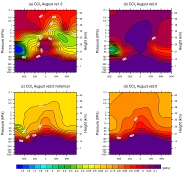
Figure 1a and b show the 1985–1990 August zonal-mean CCly values for simulations using the hybrid

advec-tion scheme without (SOCOLvs1.3) and with (SOCOLvs2) family-based mass correction. Figure 1c and d show cor-responding simulations for SOCOLvs3 using the advection scheme of Lin and Rood (1996). Since CFC surface mix-ing ratios were increasmix-ing durmix-ing this period, highest CCly

concentrations are expected in the troposphere and lowest values at the high latitudes of the stratosphere and in the mesosphere, where the air is oldest. The model deficiencies of the previous SOCOL versions mentioned in Sect. 1 are clearly visible in Fig. 1a and b: vs1.3 especially shows a very inhomogeneous stratospheric CCly distribution with a

pro-nounced minimum in the region of the southern polar vortex. In vs2, the artificial mass loss in the southern polar vortex is considerably reduced, but still present. Moreover, CCly

concentrations in the strato- and mesosphere are nearly as high as or even higher than in the troposphere. As shown in the analysis of Schraner et al. (2008), this problem is most likely caused by artificial mass transport of CClyfrom high

latitudes towards the Equator in late winter/early spring and a subsequent upward transport into the middle and upper stratosphere via the tropical pipe, due to mixing ratio gra-dients at the edges of the vortex and pipe.

Applying the scheme of Lin and Rood (1996) leads to a substantial improvement in the simulated CCly distribution

(Fig. 1c and d). However, without family-based mass fixing (Fig. 1c) we remain having an unrealistic CClyminimum in

2_NO

ysink reactions as well as stratospheric NOyproduction are

(6)

Fig. 1. Modeled zonal-mean mixing ratio of total organic plus inorganic chlorine (CCly) in August for SOCOL with resolution T31 (a) vs1.3,

(b) vs2, (c) vs3 without family correction, and (d) vs3 final version. Means calculated for the period 1985–1990.

the region of the polar vortex, but to a minor degree. Further-more, mesospheric CClymixing ratios are about 5 % smaller

than expected: tropospheric CFC concentrations were in-creasing by 0.1 ppbv yr−1 during the late 1980s; assum-ing a modeled age of air of 4 yr in the mesosphere and in the high-latitude stratosphere (Manzini and Feichter, 1999), mesospheric CClymixing ratios are estimated to be around

0.4 ppbv lower than tropospheric values, which is not the case in Fig. 1c. Applying the family-based mass correction also for the advection scheme of Lin and Rood (1996) helps overcome the problem of the artificial minimum in the re-gion of the polar vortex. In Fig. 1d the difference between tropospheric and mesospheric CClymixing ratios is as high

as expected.

Our results are corroborated by a previous study of Rasch et al. (2006), who investigated the characteristics of atmo-spheric tracer transport using a spectral, a semi-Lagrangian, and a finite volume scheme, in which all equations are ex-pressed in flux form. In this intercomparison, the finite vol-ume scheme showed the best performance: It is conservative,

less diffusive than the other schemes, and shows the highest consistency between model dynamics and tracer transport.

It is important to note that although the advection scheme of Lin and Rood (1996) itself is perfectly mass-conserving, violation of mass conservation occurs in any model with a hybrid sigmapcoordinate system like ECHAM5, where the pressure levels (and the thickness of the model layers) de-pend on the current surface pressure. This problem is caused by an inconsistency between the air mass change calculated by the advection scheme and the air mass change determined by the change in surface pressure (J¨ockel et al., 2001). In other words, the wind field, which is determined by solv-ing the basic equations in the spectral core of ECHAM5, is generally not consistent with the change of the underlying pressure grid. In ECHAM5, this so-called wind-mass incon-sistency is ignored, which may lead to a violation of global tracer mass conservation. It should be noted that the problem of wind-mass inconsistency described above only applies to pressure levels influenced by the underlying surface pres-sure. For a pressure grid defined by time-independent iso-bars, a flux-form scheme is perfectly mass-conserving. For

(7)

the sigmap-coordinate used in MA-ECHAM5, this is the case for all model layers above 75 hPa.

The violation of mass conservation for a flux-form advec-tion scheme implemented in a GCM was analyzed in detail by J¨ockel et al. (2001). They found that the problem is most critical for regions of steep gradients, e.g., at the tropopause or at the edge of the polar vortex. In the case of a homo-geneously initialized tropospheric tracer, mass loss occurred when the tracer was transported across the tropopause. A similar phenomenon is also visible in the case of CCly

with-out family-based mass correction (Fig. 1c): the upward trans-port of tropospheric CClyinto the stratosphere is clearly

un-derestimated, suggesting an artificial loss of CClyon its way

through the tropopause.

Increasing the horizontal model resolution can reduce the violation of global mass conservation, but not completely avoid it. Other approaches to deal with the mass mismatch suffer from various disadvantages: for example, simple mass fixers either lead to non-physical tracer transport or artifi-cially increase spatial gradients, and the mass-conserving grid-to-grid transformation presented by J¨ockel et al. (2001) causes an additional, non-negligible vertical diffusion.

J¨ockel et al. (2001) pointed out that despite the problems concerning mass conservation on a hybrid grid, flux-form ad-vection schemes should not be rejected, because the prob-lem of wind-mass inconsistency in principle applies also to any other advection scheme as well. In the case of a semi-Lagrangian scheme, the advection scheme itself produces an additional error in mass conservation, which in most cases exceeds that of the wind-mass inconsistency. Figure 1 con-firms that switching from a semi-Lagrangian scheme to the advection scheme of Lin and Rood (1996) leads to an enor-mous improvement, even without family-based mass correc-tion. The best way to avoid the problem of wind-mass incon-sistency would be a grid-point dynamical core instead of the presently used spectral core. This approach has been already implemented in several CCMs (e.g., WACCM, GEOSCCM). The joint ICON project of the MPI for Meteorology in Ham-burg and the Deutscher Wetterdienst (DWD) aims at devel-oping a dynamical core that solves the equations of motion in grid-point space (http://www.mpimet.mpg.de/en/science/ models/icon.html).

5 Evaluation of SOCOLvs3

Subsequently we evaluate the new model version SOCOLvs3 by comparing with observations and with SOCOLvs2, fo-cusing on stratospheric dynamics and chemistry. SOCOLvs2 was extensively evaluated within CCMVal-2 (SPARC, 2010). A detailed description of SOCOLvs2 is given in Schraner et al. (2008). The SOCOLvs2 simulations are identical to the CCMVal-2 REF-B1 scenario; i.e., they cover the time period 1960–2005. The boundary conditions are mostly identical to the SOCOLvs3 simulations. For SOCOLvs2 three ensemble

members (T31) are available, whereas for SOCOLvs3 we use one realization for each horizontal resolution, T31 and T42. An overview of the applied diagnostics and the respective reference datasets is given in Table 1.

5.1 Stratospheric dynamics

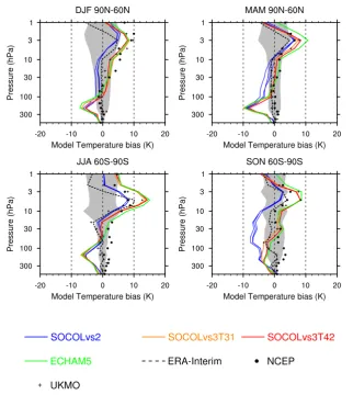
Following previous CCMVal assessments (Eyring et al., 2006; SPARC, 2010), we compare simulated stratospheric temperatures with the ERA-40 (Uppala et al., 2005) and ERA-Interim (Simmons et al., 2006) reanalyses as well as the NCEP (Gelman et al., 1996) and UKMO (Swinbank and O’Neill, 1994) stratospheric analyses. The mean winter and spring temperature biases in polar regions are shown in Fig. 2. In the lowermost stratosphere (LMS) both SOCOL versions show a cold bias of comparable magnitude. Run-ning SOCOLvs3 in T42 horizontal resolution reduces the cold bias in the LMS of both hemispheres by 1–2 K. The largest temperature bias (−10 K) is found in the northern LMS in spring, whereas in the Southern Hemisphere (SH) spring both model versions perform similarly, with a bias of about−4 K. It should be noted that the described cold bias is a widespread feature of CCMs (Eyring et al., 2006; SPARC, 2010). The reasons for the cold bias are not yet fully under-stood and might differ between different models (e.g., Paw-son et al., 2000). For example, Stenke et al. (2008) found that the cold bias in the CCM E39C was partly caused by a severe wet bias in the extratropical LMS, resulting in an excessive longwave cooling.

Between 100 and 10 hPa the comparison can be summa-rized as follows: in the NH all model versions expect SO-COLvs2 during springtime lie within the±1 standard devi-ation range of ERA-40, with SOCOLvs3 simulating slightly higher temperatures than SOCOLvs2. During SH winter all versions show a good agreement with ERA-40. In SH spring SOCOLvs3 again lies within the ERA-40 interannual vari-ability, whereas SOCOLvs2 is significantly colder (the “cold pole” problem). It is clear that this improvement by several degrees Kelvin is related to and has repercussions for the simulation of the Antarctic ozone hole.

(8)

Table 1. Diagnostics and observational data used in this study.

Process Diagnostics Observations

Dynamics High-latitude temperature biases (Fig. 2) ERA-40 (Uppala et al., 2005), ERA-Interim (Simmons et al., 2006),

NCEP, UKMO Reanalyses (Eyring et al., 2006)

Easterlies at 60◦S (Fig. 3) ERA-40, ERA-Interim

Heat flux 100 hPa (Fig. 4) ERA-40, NCEP

Transport Vertical and latitudinal profiles of CH4(Fig. 6) HALOE (Grooß and Russell, 2005)

Tape recorder (Fig. 8) HALOE

UTLS Seasonal cycle ofT and H₂O, 100 hPa, Eq (Fig. 5) ERA-40, ERA-Interim, HALOE

Chemistry Vertical and latitudinal profiles of H2O (Fig. 7), HALOE

Cl species (Fig. 9), O₃(Fig. 10)

Total ozone column (Fig. 11) NIWA (Bodeker et al., 2005)

Fig. 2. Climatological mean (1980–1999) temperature biases relative to the ERA-40 reanalysis for 60–90◦N (top) and 60–90◦S (bottom) during winter (left) and spring (right). Biases are calculated for SOCOLvs2 (blue lines, 3 ensemble members), SOCOLvs3 T31 horizontal resolution (orange line), SOCOLvs3 T42 horizontal resolution (red line), MA-ECHAM5 T31 horizontal resolution (green line) and for ERA-Interim (dashed black line, 1989–1999), NCEP (dots, 1980–1999) and UKMO (crosses, 1992–2001) reanalyses. The grey area shows ERA-40 plus and minus 1 standard deviation about the climatological mean.

(9)

ozone absorption in the stratosphere (Cagnazzo et al., 2007). The modifications applied to the radiation scheme lead to a significant warming of almost the entire middle atmosphere, with the strongest temperature increase of about 6 K at the summer stratopause. The higher stratospheric temperatures are in better agreement with the NCEP analysis that was used by Cagnazzo et al. (2007) for model evaluation. These changes in the shortwave radiation scheme might explain a part of the warming of the upper stratosphere in SOCOLvs3. However, it should be mentioned that the pure GCM MA-ECHAM5, without coupled chemistry (green line in Fig. 2), shows similar temperature biases in the polar winter strato-sphere to SOCOLvs3. During other seasons (spring and sum-mer, not shown) MA-ECHAM5 shows up to 5 K higher tem-peratures in the upper stratosphere. These differences are most probably related to different stratospheric water vapor concentrations: since MA-ECHAM5 does not include chem-ical water vapor production, upper-stratospheric water vapor concentrations in MA-ECHAM5 are 2–3 ppmv lower than in SOCOLvs3, resulting in less longwave cooling in MA-ECHAM5. Comparing stratospheric ozone distributions in MA-ECHAM5 and SOCOLvs3 reveals largest differences in polar fall and winter. During this time shortwave heating by ozone is negligible in polar regions, indicating that the speci-fication of the ozone distribution (fixed ozone versus interac-tively coupled ozone) has only a minor impact on simulated temperatures in the polar stratosphere.

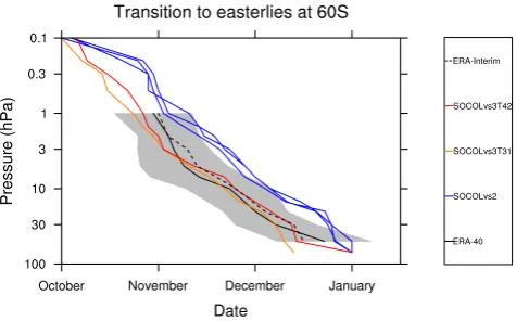
The pronounced “cold pole” problem seen in SOCOLvs2 is associated with a stronger polar vortex and a delayed breakdown of the vortex, both of which affect the simula-tion of the Antarctic ozone hole. This model behavior is re-flected in the seasonal cycle of the zonal winds and a delayed transition from westerlies to easterlies at 60◦_{S (Fig. 3). In}

agreement with the improved representation of stratospheric temperatures in SOCOLvs3 (Fig. 2, bottom right), the timing of the simulated zonal wind reversal in SOCOLvs3 compares very well with ERA-40 and ERA-Interim (Fig. 3).

Stratospheric polar temperatures during winter and spring as well as their interannual variability are largely determined by the forcing of planetary waves that propagate from the troposphere into the stratosphere. Newman et al. (2001) have shown that the polar temperatures in late winter at 50 hPa are well correlated with the meridional heat flux at 100 hPa in the middle of winter. The meridional heat flux at 100 hPa is proportional to the vertical component of the Eliassen–Palm (EP) flux entering the stratosphere and therefore a measure of transferred wave energy. Figure 4 compares the model re-sults for SOCOLvs2 and SOCOLvs3 with the ERA-40 and NCEP reanalyses. The slope and the intercept of the regres-sion lines (see legend of Fig. 4) provide additional informa-tion about the model behavior: the slope indicates the strato-spheric temperature response to a unit amount of resolved tropospheric wave forcing. The intercept indicates the polar stratospheric temperature if no resolved wave-driving were present. In the NH SOCOLvs2 shows the best performance

Fig. 3. Timing of transition from westerlies to easterlies (indicat-ing the breakdown of the Antarctic vortex) at 60◦S for ERA-40 (solid black line), ERA-Interim (dashed black line), SOCOLvs2 (blue lines), SOCOLvs3 T31 horizontal resolution (orange line), and SOCOLvs3 T42 horizontal resolution (red line). Grey shading indicates ERA-40 plus and minus 1 standard deviation about the climatological mean (1980–1999).

of the three model versions in terms of slope and intercept, with a small vertical offset reflecting the simulated cold bias (Fig. 2). The simulated temperature response per unit of wave forcing is in good agreement with ERA-40. The results for SOCOLvs3 show a displacement to the right, suggesting that a larger amount of tropospheric wave forcing is required in SOCOLvs3 to simulate stratospheric temperatures compara-ble to ERA-40. However, the linear fit parameters of both model versions, SOCOLvs2 and SOCOLvs3, still lie within the 95 % confidence interval of ERA-40 (not shown).

In the SH the model results show larger variation, espe-cially with respect to the slope of the regression lines. Again SOCOLvs2 is displaced below the reanalysis, reflecting a small cold temperature bias. In terms of the simulated tem-perature response to the wave forcing, SOCOLvs2 shows an underestimated sensitivity, while SOCOLvs3, especially the T42 version, overestimates the temperature response. SO-COLvs3 in T31 resolution compares best with ERA-40.

(10)

10 A. Stenke et al.: The SOCOL version 3.0 chemistry–climate model

(b) (a)

()v 0T0) [K ms−1] at 100 hPa (averaged over 40◦N to 80◦N for January and February) versus temperatures [K] at 50 hPa (averaged over 60◦N to 90◦N for February and March). Shown are 20 yr from 1980 to 1999 for SOCOLvs3 T42 (red), SOCOLvs3 (orange), SOCOLvs2 (blue), ERA-40 (black) and NCEP (grey) reanalyses. Right: same for Southern Hemisphere with heat fluxes at 100 hPa averaged over 40◦S to 80◦S for July and August versus temperatures at 50 hPa averaged over 60◦S to 90◦S for August and September.

Fig

(a)

(b)

. 5. Seasonal variation of the climatological mean temperature (left) and H₂O (right) at 100 hPa at the Equator, for SOCOLvs2 (blue lines), SOCOLvs3 T31 horizontal resolution (orange line), SOCOLvs3 T42 horizontal resolution (red line), ERA-40 (solid black line) and

ERA-Interim (dashed black line, grey shading±1σ, 1992–2001), and HALOE observations (solid black line, grey shading±1σ, 1992– 2001).

agreement with ERA-Interim. As a consequence of the tem-perature increase at the equatorial tropopause, SOCOLvs3 simulates higher water vapor mixing ratios at this level than SOCOLvs2, especially during early summer (Fig. 5, right). Although both SOCOL versions simulate the maximum wa-ter vapor mixing ratios one month earlier than observed, the absolute values compare very well with HALOE. Minimum water vapor mixing ratios, however, are overestimated by SOCOL. Gettelman et al. (2009) (see also SPARC, 2010) examined the dehydration process at the tropical tropopause and the role of the cold point temperature by calculating the correlation between the saturation water vapor mixing ratio at cold point temperature (QSAT(TCPT)) and the water vapor

mixing ratio at or just above the tropical tropopause. The

re-spective values for all SOCOL versions indicate higher mean saturation levels (about 80 %) of air masses entering the stratosphere than those derived from ERA-Interim/HALOE (about 70 %).

5.2 Methane

The stratospheric methane (CH4) distribution is largely

con-trolled by methane oxidation and transport. Due to its long photochemical lifetime, methane is an excellent tracer of at-mospheric circulation.

Figure 6 shows climatological mean mixing ratios of methane from SOCOLvs2 and vs3 (T31, T42) and HALOE observations (Grooß and Russell, 2005). For Fig. 6 CH4on

equivalent latitudes has been used. In the middle and upper

Geosci. Model Dev., 6, 1–22, 2013 www.geosci-model-dev.net/6/1/2013/

Fig. 4. (a) Heat fluxes (v0_T0_{) [K ms}−1_{] at 100 hPa (averaged over 40}◦_{N to 80}◦_{N for January and February) versus temperatures [K] at} 50 hPa (averaged over 60◦N to 90◦N for February and March). Shown are 20 yr from 1980 to 1999 for SOCOLvs3 T42 (red), SOCOLvs3 (orange), SOCOLvs2 (blue), ERA-40 (black) and NCEP (grey) reanalyses. (b) Same for Southern Hemisphere with heat fluxes at 100 hPa averaged over 40◦S to 80◦S for July and August versus temperatures at 50 hPa averaged over 60◦S to 90◦S for August and September.

10 A. Stenke et al.: The SOCOL version 3.0 chemistry–climate model

(b) (a)

()v 0T0) [K ms−1] at 100 hPa (averaged over 40◦N to 80◦N for January and February) versus temperatures [K] at 50 hPa (averaged over 60◦N to 90◦N for February and March). Shown are 20 yr from 1980 to 1999 for SOCOLvs3 T42 (red), SOCOLvs3 (orange), SOCOLvs2 (blue), ERA-40 (black) and NCEP (grey) reanalyses. Right: same for Southern Hemisphere with heat fluxes at 100 hPa averaged over 40◦S to 80◦S for July and August versus temperatures at 50 hPa averaged over 60◦S to 90◦S for August and September.

Fig

(a)

(b)

. 5. Seasonal variation of the climatological mean temperature (left) and H₂O (right) at 100 hPa at the Equator, for SOCOLvs2 (blue lines), SOCOLvs3 T31 horizontal resolution (orange line), SOCOLvs3 T42 horizontal resolution (red line), ERA-40 (solid black line) and

ERA-Interim (dashed black line, grey shading±1σ, 1992–2001), and HALOE observations (solid black line, grey shading±1σ, 1992– 2001).

agreement with ERA-Interim. As a consequence of the tem-perature increase at the equatorial tropopause, SOCOLvs3 simulates higher water vapor mixing ratios at this level than SOCOLvs2, especially during early summer (Fig. 5, right). Although both SOCOL versions simulate the maximum wa-ter vapor mixing ratios one month earlier than observed, the absolute values compare very well with HALOE. Minimum water vapor mixing ratios, however, are overestimated by SOCOL. Gettelman et al. (2009) (see also SPARC, 2010) examined the dehydration process at the tropical tropopause and the role of the cold point temperature by calculating the correlation between the saturation water vapor mixing ratio at cold point temperature (Q_SAT(T_CPT)) and the water vapor mixing ratio at or just above the tropical tropopause. The

re-spective values for all SOCOL versions indicate higher mean saturation levels (about 80 %) of air masses entering the stratosphere than those derived from ERA-Interim/HALOE (about 70 %).

5.2 Methane

equivalent latitudes has been used. In the middle and upper

Geosci. Model Dev., 6, 1–22, 2013 www.geosci-model-dev.net/6/1/2013/ Fig. 5. Seasonal variation of the climatological mean temperature (a) and H2O (b) at 100 hPa at the Equator, for SOCOLvs2 (blue lines),

SOCOLvs3 T31 horizontal resolution (orange line), SOCOLvs3 T42 horizontal resolution (red line), 40 (solid black line) and ERA-Interim (dashed black line, grey shading±1σ, 1992–2001), and HALOE observations (solid black line, grey shading±1σ, 1992–2001).

agreement with ERA-Interim. As a consequence of the tem-perature increase at the equatorial tropopause, SOCOLvs3 simulates higher water vapor mixing ratios at this level than SOCOLvs2, especially during early summer (Fig. 5b). Al-though both SOCOL versions simulate the maximum water vapor mixing ratios one month earlier than observed, the ab-solute values compare very well with HALOE. Minimum water vapor mixing ratios, however, are overestimated by SOCOL. Gettelman et al. (2009) (see also SPARC, 2010) examined the dehydration process at the tropical tropopause and the role of the cold point temperature by calculating the correlation between the saturation water vapor mixing ratio at cold point temperature (QSAT(TCPT)) and the water vapor

mixing ratio at or just above the tropical tropopause. The re-spective values for all SOCOL versions indicate higher mean saturation levels (about 80 %) of air masses entering the

stratosphere than those derived from ERA-Interim/HALOE (about 70 %).

5.2 Methane

equivalent latitudes has been used. In the middle and upper tropical and subtropical stratosphere SOCOLvs3 shows a general reduction of CH4 compared to the previous model

version (Fig. 6b), resulting in better agreement with the

(11)

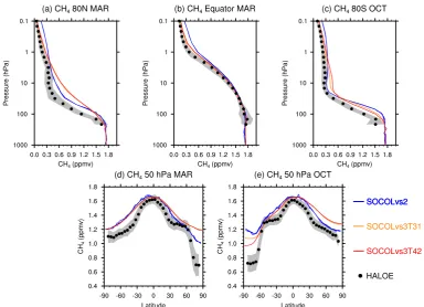
Fig. 6. Comparison of climatological (1992–2001) zonal-mean CH4mixing ratios (ppmv) from SOCOL and from HALOE for the same

equivalent latitude. Upper panels: vertical profiles at (a) 80◦N, March; (b) 0◦, March; and (c) 80◦S, October. Lower panels: meridional cross-section at 50 hPa in (d) March and (e) October. The grey shaded areas indicate the HALOE standard deviation (±1σ).

HALOE measurements. A slower residual circulation in SO-COLvs3 (see also Sect. 5.3), and therefore a more efficient CH4oxidation during ascent, can explain this finding. In the

lower-stratosphere northern extratropics, SOCOLvs3 gener-ally simulates higher CH4mixing ratios than vs2. A similar

difference pattern in the lower stratosphere is also found for N2O and the CFCs.

Remarkable differences in the simulated CH4distribution

of both model generations also occur in the southern po-lar vortex (Fig. 6e), with SOCOLvs3 showing significantly lower CH4 values than SOCOLvs2 and, therefore, a much

better agreement with the HALOE observations. This im-provement is most pronounced in the T42 simulation. The high CH4 concentrations in SOCOLvs2 are most probably

related to the semi-Lagrangian transport scheme, which is known to be excessively diffusive in the presence of sharp gradients; i.e., there is an artificial horizontal diffusion of CH4-rich air masses from mid-latitudes into the polar

vor-tex. Further artifacts from the application of the mass fixer can also not be excluded. Possible reasons for the remain-ing high CH4 bias in SOCOLvs3 are too-strong horizontal

mixing across the vortex edge and/or too-weak downward transport in the high latitudes. It should be mentioned that most of the CCMVal models showed a similar behavior to SOCOLvs3 in the Southern Hemisphere polar spring (see

Fig. 5 of Eyring et al., 2006). Due to limited observations in polar regions and the large year-to-year variability in the Arctic, there is also considerable uncertainty associated with the HALOE data, which could be partly responsible for the apparently large discrepancy at latitudes north of 70◦N.

5.3 Water vapor

There are two sources of H2O in the stratosphere: upward

transport from the troposphere and CH4 oxidation in the

stratosphere. The amount of tropospheric water vapor enter-ing the stratosphere is directly related to the cold point tem-perature at the tropical tropopause. The annual cycle in the tropical tropopause temperature (Fig. 5a) generates a corre-sponding signal in the tropical water vapor, which slowly propagates upward in the tropical pipe (the so-called wa-ter vapor “tape recorder”; Mote et al., 1996). The “tape recorder” signal can be used to assess both the ascent rate in the tropical pipe by the residual circulation and the mixing with mid-latitude air.

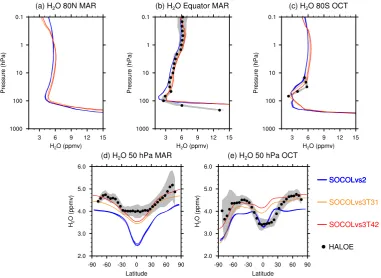
Figure 7 compares mean vertical profiles of H2O at

(12)

Fig. 7. Same as in Fig. 6 but for water vapor in ppmv.

a general increase in stratospheric water vapor mixing ra-tios compared to vs2. Another reason is the slowdown of the Brewer–Dobson circulation, which leads to enhanced wa-ter vapor production by CH4oxidation. In agreement with a

stronger warming of the tropical tropopause (Fig. 5a), the in-crease in stratospheric water vapor is more pronounced in the T42 simulation.

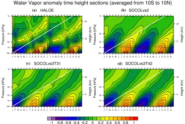
SOCOLvs3 compares well with observations throughout the stratosphere with the exception of the lower tropical stratosphere. Compared to HALOE, SOCOLvs3 is slightly too moist (up to 10 %) but agrees well with MIPAS measure-ments, which are around 10 % moister than HALOE (Milz et al., 2009; not shown). In the lower tropical stratosphere, the model bias depends on pressure level and season. The rea-son is obvious from the water vapor tape recorder displayed in Fig. 8: while the seasonal water vapor cycle at the tropi-cal tropopause at 100 hPa is well captured by the model, the upward propagation of the tape recorder signal is too fast in all model versions. At 50 hPa, the simulated annual cy-cle is 4.5 months out of phase compared to HALOE. The HALOE tape recorder signal propagates with a phase speed of about 10 km yr−1, while the propagation speed in SOCOL is twice as fast, with values of 21.8 km yr−1 in SOCOLvs2 and 18.5 km yr−1 (19.9 km yr−1) in SOCOLvs3T31 (T42). The clear overestimation of the upward transport in the trop-ical pipe shown by the tape recorder suggests a residual cir-culation that is too strong in SOCOL. Struthers et al. (2009) found that the stratospheric air in SOCOLvs2 is 1–2.5 yr too

young. Compared with SOCOLvs2, the tape recorder indi-cates a slowdown of the residual circulation in vs3 by 10– 15 %, but the vertical propagation is still too fast. The prob-lem of a too-fast upward transport in the tropical pipe seems to be a common problem of ECHAM-based CCMs (see e.g. Fig. 8 of Eyring et al., 2006; SPARC, 2010). With respect to the decay of the amplitude with height due to mixing processes, i.e., the vertical attenuation of the tape recorder signal, SOCOLvs2 shows a too-rapid decay in the middle stratosphere, indicating a strong tropical–extratropical mix-ing. SOCOLvs3 agrees slightly better with the HALOE ob-servations.

5.4 Chlorine species/HCl

Figure 9 shows simulated total inorganic plus organic chlo-rine (CCly), total inorganic chlorine (Cly) and reactive

chlo-rine (ClOx) as well as simulated and observed HCl for the

1990s. The improvement in simulated CCly due to the

ad-vanced advection scheme of Lin and Rood (1996) described in Sect. 4 is clearly visible: while SOCOLvs2 shows an un-realistic S-shape in the vertical CCly profiles with a

mini-mum around 20 km during polar winter and early spring, vs3 shows the expected CClydecrease with height and latitude;

i.e., older air masses contain less CCly in accordance with

increasing CFC surface mixing ratios until the early 1990s. The improved conservation of the CClyfamily leads also

to an improved representation of HCl in the model. In the

(13)

Fig. 8. Averaged (1992–2001) time–height sections of water vapor mixing ratio shown as the deviation from the mean profile, averaged between 10◦N and 10◦S for

(a)

HALOE,

(b)

SOCOLvs2, (c)

SOCOLvs3 T31, and (d)

SOCOLvs3 T42. Two consecutive (identical) cycles are shown. The white line indicates the phase speed of the HALOE tape recorder signal.

i.e., older air masses contain less CCly in accordance with

increasing CFC surface mixing ratios until the early 1990s. The improved conservation of the CClyfamily leads also

to an improved representation of HCl in the model. In the lower stratosphere (50 hPa) SOCOLvs3 compares well with HALOE HCl measurements except at southern high latitudes in winter and spring (Fig. 9c and e). This is related to a downward shift of the HCl and Cly profiles inside the

po-lar vortex (Fig. 9c) in SOCOLvs3 compared to vs2. In the middle stratosphere, the model bias is reduced, but simu-lated HCl remains too high (Fig. 9b). This problem might be related to an incorrect chlorine partitioning: in the mid-dle stratosphere, simulated ClONO2is underestimated by up

to 40 % compared to retrievals of the Cryogenic Limb Ar-ray Etalon Spectrometer (CLAES) (Roche et al., 1993, 1994) (not shown). This may partly be explained by an underesti-mation of stratospheric NOxresulting in a too-slow ClONO2

formation through the reaction of ClO with NO2.

For reactive chlorine species (ClOx), the difference pattern

between the two model versions is more complicated. In the tropical middle and upper stratosphere, ClOx simulated by

SOCOLvs3 is remarkably higher than for vs2 (Fig. 9b). This can be explained by a general decrease of stratospheric NOx

(and NOy) in vs3 compared to SOCOLvs2 (not shown),

re-sulting in a slower ClOxdeactivation by the reaction of ClO

with NO2. In the southern polar vortex, ClOxis almost

dou-ble in winter (not shown), but lower in spring (Fig. 9c and e). The former can be explained by the increase of Clyin the

same region, while the latter could be the effect of substan-tially lower ozone concentrations in late August and Septem-ber leading to a higher conversion of Cl to the reservoir gas HCl, as there is less ozone left to react with.

Increasing the model resolution from T31 to T42 signif-icantly affects the chlorine concentration in the polar vor-tex. Both Clyand HCl are increased for T42, which is

prob-ably the effect of a more efficient transport barrier at the vortex edge and less horizontal mixing. In contrast, ClOx

concentrations in the southern polar vortex are hardly in-fluenced (Fig. 9a and d), probably because of two compen-sating effects: while Clyis increased, the chlorine activation

on PSC II is decreased due to a warmer polar vortex. In the northern polar vortex, the T42 model version shows a ClOx

reduction of 40–80 %, as chlorine activation on STSs is sub-stantially reduced due to the higher temperatures.

5.5 Ozone

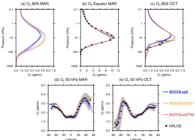
Figure 10 shows mean vertical profiles of O3 at different

latitudes as well as latitudinal distributions at 50 hPa from both model versions and measurements. At 50 hPa, the differ-ences in simulated ozone mixing ratios between both model versions are rather small, with SOCOLvs3 showing slightly higher ozone values. The horizontal resolution has almost no impact on the simulated ozone distribution in SOCOLvs3. The largest differences occur in the northern high latitudes, especially during spring, where SOCOLvs3 simulates sig-Fig. 8. Averaged (1992–2001) time–height sections of water vapor mixing ratio shown as the deviation from the mean profile, averaged between 10◦N and 10◦S for (a) HALOE, (b) SOCOLvs2, (c) SOCOLvs3 T31, and (d) SOCOLvs3 T42. Two consecutive (identical) cycles are shown. The white line indicates the phase speed of the HALOE tape recorder signal.

lower stratosphere (50 hPa) SOCOLvs3 compares well with HALOE HCl measurements except at southern high latitudes in winter and spring (Fig. 9c and e). This is related to a downward shift of the HCl and Cly profiles inside the

po-lar vortex (Fig. 9c) in SOCOLvs3 compared to vs2. In the middle stratosphere, the model bias is reduced, but simu-lated HCl remains too high (Fig. 9b). This problem might be related to an incorrect chlorine partitioning: in the mid-dle stratosphere, simulated ClONO2is underestimated by up

to 40 % compared to retrievals of the Cryogenic Limb Ar-ray Etalon Spectrometer (CLAES) (Roche et al., 1993, 1994) (not shown). This may partly be explained by an underesti-mation of stratospheric NOxresulting in a too-slow ClONO2

formation through the reaction of ClO with NO2.

For reactive chlorine species (ClOx), the difference pattern

between the two model versions is more complicated. In the tropical middle and upper stratosphere, ClOx simulated by

SOCOLvs3 is remarkably higher than for vs2 (Fig. 9b). This can be explained by a general decrease of stratospheric NOx

(and NOy) in vs3 compared to SOCOLvs2 (not shown),

re-sulting in a slower ClOxdeactivation by the reaction of ClO

with NO2. In the southern polar vortex, ClOxis almost

dou-ble in winter (not shown), but lower in spring (Fig. 9c and e). The former can be explained by the increase of Clyin the

same region, while the latter could be the effect of substan-tially lower ozone concentrations in late August and Septem-ber leading to a higher conversion of Cl to the reservoir gas HCl, as there is less ozone left to react with.

Increasing the model resolution from T31 to T42 signif-icantly affects the chlorine concentration in the polar vor-tex. Both Clyand HCl are increased for T42, which is

prob-ably the effect of a more efficient transport barrier at the vortex edge and less horizontal mixing. In contrast, ClOx

concentrations in the southern polar vortex are hardly in-fluenced (Fig. 9a and d), probably because of two compen-sating effects: while Clyis increased, the chlorine activation

on PSC II is decreased due to a warmer polar vortex. In the northern polar vortex, the T42 model version shows a ClOx

reduction of 40–80 %, as chlorine activation on STSs is sub-stantially reduced due to the higher temperatures.

5.5 Ozone

Figure 10 shows mean vertical profiles of O3 at different

(14)

Fig. 9. Same as in Fig. 6 but for various chlorine species in ppbv. Dashed lines: odd chlorine (ClOx); dotted lines: total inorganic chlorine

(Cly); dash-dotted lines: total inorganic plus organic chlorine (CCly); filled circles: HCl.

directly related to the simulated distribution of the chlorine species (Fig. 9c). This feature is no longer apparent in SO-COLvs3.

In the tropical stratosphere SOCOLvs3 (T31, T42) com-pares very well with HALOE observations (Fig. 10b), but slightly (∼5 %) overestimates the observations at high al-titudes. In the lower stratosphere, simulated ozone in SO-COLvs3 is positively biased, but within the standard devi-ation of the observdevi-ations in most regions (Fig. 10d and e).

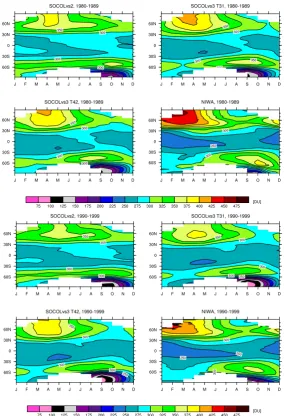
Finally, Fig. 11 shows monthly zonal-mean total ozone for the 1980–1989 and 1990–1999 periods. While SOCOLvs2 was not able to reproduce the seasonal cycle in tropical and mid-latitudinal regions, the seasonal variability in SO-COLvs3 agrees well with the observations. The improve-ment of the seasonal variability of total ozone in vs3 is a direct effect of the substantial changes of ozone in the low-ermost stratosphere due to the advection scheme of Lin and Rood (1996) as described above. The timing of the Antarc-tic ozone hole (middle of September instead of beginning of October) is now in good agreement with observations, whereas the spring maximum in southern mid-latitudes oc-curs about 2 months earlier than observed. The ozone hole in SOCOLvs3 is clearly too deep, which is a degradation

compared to SOCOLvs2. However, the higher total ozone values in vs2 during the ozone hole period are not the result of an overall better model performance, but related to the un-realistic high ozone concentrations in the polar lowermost stratosphere (Fig. 10c). The vs3 model bias in total ozone in the polar region is less pronounced in the T42 simulation. In northern polar winter and spring, all model versions are neg-atively biased, with SOCOLvs3 in T42 horizontal resolution again comparing best with observations. In the high latitudes of both summer hemispheres, SOCOLvs3 shows a reduced model bias in total ozone. Both model versions reproduce the observed negative trend in total column ozone at mid-and high latitudes. Overall, the representation of total column ozone has clearly improved from SOCOLvs2 to vs3, with the T42 simulation showing a slightly better agreement with ob-servations than the T31 simulation. For a better comparison, Fig. 12 shows the differences in monthly zonal-mean total ozone between SOCOL and NIWA for the 1980–1989 and 1990–1999 periods.

5.6 Grading

We illustrate the benefits of the new model version by applying the grading technique proposed by Waugh and

(15)

Fig. 10. Same as in Fig. 6 but for ozone in ppmv.

Eyring (2008). This method is based on the comparison of several quantities extracted from the model output with ob-servations, taking into account the internal variability and uncertainties of the observational data. These model vali-dation metrics provide a quick overview on the progress in model development. However, it should be noted that there has also been criticism (e.g., Grewe and Sausen, 2009) point-ing to specific weaknesses in this method concernpoint-ing sta-tistical limitations of the grading method. Furthermore, as stated by Butchart et al. (2011), metrics themselves provide only limited information on the quality of simulated phys-ical processes and, therefore, need to be combined with a comprehensive analysis of model results, as was done in the previous sections. Notwithstanding these limitations, similar validation metrics were also applied in SPARC (2010), ex-ploiting however a more complicated set of parameters and procedures. Reproducing all metrics from SPARC (2010) would go beyond the scope of this paper. We therefore cal-culate the grades (g) using the original Eq. (4) of Waugh and Eyring (2008) in the following form:

g=max

0,

1−abs(fm−fobs) 3sobs

, (1)

wherefmandfobsare the model and observational values of

each considered quantity andsobsis the interannual standard

deviation of the observations. The set of considered quanti-ties consists of 16 variables listed in Table 2 of Waugh and

Eyring (2008). The observed climatological mean and inter-annual standard deviation of considered quantities were cal-culated using ERA-40 (Uppala et al., 2005) for the period 1980–1999 and HALOE UARS data (Grooß and Russell, 2005) for the period 1991–2000, while the mean ages data were taken from Eyring et al. (2006). The grading marks for all considered quantities, as well as the overall model grade defined as the mean over all grades, are shown in Fig. 13 for SOCOLvs2 as well as SOCOLvs3 with horizontal trun-cation at T31 and T42. As described in Sect. 2 the main dif-ference between the two model versions is of the applica-tion of MA-ECHAM5 instead of MA-ECHAM4 as the core GCM and the flux-form semi-Lagrangian transport scheme (Lin and Rood, 1996) instead of a hybrid transport scheme (Zubov et al., 1999). The chemical module remains the same. The application of the new transport scheme leads to a sub-stantial improvement of the model performance in the sim-ulation of the total inorganic chlorine and methane over the southern high latitudes in October (Cly-SP and CH4-SP) as

(16)

Fig. 11. Zonal mean of total ozone in DU averaged over the two 10 yr periods, 1980–1989 (upper four panel) and 1990–1999 (lower four panel), for SOCOLvs2, SOCOLvs3 in T31 and T42 horizontal resolution, and NIWA observational data.

used for calculating the age of air in SOCOLvs2 and SO-COLvs3, respectively. Within SOCOLvs3 we used a passive CO2 tracer. As a lower boundary condition we prescribed

monthly and zonal-mean CO2mixing ratios including a

lin-ear trend of 1.5 ppmv yr−1together with a climatological but latitudinally varying seasonal cycle (Hall and Prather, 1993). In SOCOLvs2 we applied a similar procedure, but instead of a seasonally varying CO2-like tracer we used a passive tracer

with a global mean, linearly increasing lower boundary con-dition.

The application of the new GCM core improved the rep-resentation of polar temperatures in the lower stratosphere, while the representation of the heat flux in the NH remains almost unchanged and got even worse in the SH. The over-all grade demonstrates the slightly improved performance of

the new model version, confirming that the model develop-ment is heading in the right direction. However, it is not clear whether the change of an overall grade from∼0.55 to∼0.65 is significant (Grewe and Sausen, 2009). Furthermore, the overall grade might change with the chosen subset of pa-rameters and diagnostics. Future efforts should aim at the improvement of the performance of SOCOL in the tropical lower stratosphere, where the representation of the tempera-ture and water vapor distribution, as well as the mean age of air, are still not satisfactory. As was mentioned by Butchart et al. (2011), the grading simply illustrates the model per-formance, but it does not provide substantial information re-garding missing or under-represented processes, so that a more careful analysis of the model runs is necessary to define which part of the model can and should be improved.

(17)

Fig. 12. Differences of zonal-mean total ozone between the different SOCOL simulations and NIWA observations averaged over the two 10 yr periods, 1980–1989 (left) and 1990–1999 (right).

6 Conclusions

This paper presents the third generation of the coupled chemistry–climate model SOCOL. Compared to the previ-ous model version, the underlying general circulation model has been updated from MA-ECHAM4 to MA-ECHAM5, and the former hybrid advection algorithm has been re-placed by a mass-conserving and shape-preserving flux-form semi-Lagrangian scheme. In contrast to its predecessors SO-COLvs3 is now fully parallelized and can be used on multi-processor machines. Stratospheric model dynamics and sim-ulated distributions of chemical trace species have been eval-uated against various observational datasets and previous model versions. The previous model version SOCOLvs2 was extensively validated within CCMVal-2 (SPARC, 2010). In the following we summarize the model performance of SO-COLvs2 and SOCOLvs3 with respect to stratospheric dy-namics, transport, and ozone chemistry. Statements in quotes refer to SOCOLvs2 (SPARC, 2010):

“SOCOLvs2 simulates the stratospheric mean state in winter and spring well in both hemispheres al-though there are significant biases in the SH lower stratosphere in spring. Stratospheric variability in the model is weak, perhaps linked to the small amounts of heat flux at 100 hPa. In the SH the relationship between heat flux and lower strato-spheric temperatures is well simulated”.