R
EGULARA
RTICLEA study of the construction of the correlation matrix
of
241
Pu(nth,f) isobaric
fi
ssion yields
Sylvain Julien-Laferrière1,2,*, Abdelaziz Chebboubi1, Grégoire Kessedjian2, and Olivier Serot1
1
CEA, DEN, DER, SPRC, 13108 Saint-Paul-Lez-Durance, France 2
LPSC, Université Grenoble-Alpes, CNRS/IN2P3, 38026 Grenoble, France
Received: 6 December 2017 / Received infinal form: 20 March 2018 / Accepted: 25 May 2018
Abstract.Two blind analyses for241Pu(nth,f) isobaricfission yields have been conducted, one analysis using a mix of a Monte-Carlo and an analytical method, the other one relying only on analytical calculations. The calculations have been derived from the same analysis path and experimental data, obtained on the LOHENGRIN mass spectrometer at the Institut Laue-Langevin. The comparison between the two analyses put into lights several biases and limits of each analysis and gives a comprehensive vision on the construction of the correlation matrix. It gives confidence in the analysis scheme used for the determination of thefission yields and their correlation matrix.
1 Introduction
Nuclearfission yields are key parameters for understanding the fission process [1] and to evaluate reactor physics quantities, such as decay heat [2]. Despite a sustained effort allocated tofission yields measurements and code develop-ment, the recent evaluated libraries (JEFF-3.3 [3], ENDF/ B-VII.1 [4],…) still present shortcomings, especially in the reduction of the uncertainties and the presence of reliable variance-covariance matrices. Yet these matrices are compulsory to use nuclear data, in particular when it comes to propagate uncertainties. A collaboration among the French Alternative Energies and Atomic Energy Commission (CEA), the Laboratory of Subatomic Physics and Cosmology (LPSC) and the Institut Laue-Langevin (ILL), started in 2009, aims at tackling these issues by providing precise measurements offission yields with the related experimental covariance matrices for major actinides [5]. In particular for the 241Pu nuclide which is a major isotope in the context of multi-recycling and which is investigated in the present work.
Two measurements for thermal neutron inducedfission of 241Pu have been carried out at the ILL in Grenoble (France), using the LOHENGRIN mass spectrometer [6,7] in May 2013 [8], labelled as Exp.1, and November 2015 [9], labelled as Exp.2. This instrument allows a selection of fission products regarding the A/q and Ek/q ratios, supplying an ion beam of of mass A, kinetic energy Ek and of ionic charge q with an excellent mass resolution
(DA/A≃1/400). A double ionization chamber with a Frisch grid, similar to the one used in [10], is used to measure the count rate N(A, t, Ek, q). The entire heavy peak region has been measured as well as a significant number of light masses.
The analysis scheme for the high yields region1(85–111 for the light masses and 130–151 for the heavy masses) has been subjected to two independent blind analyses [11], from the same raw data and analysis scheme.
The first one relies on a Monte-Carlo (MC) approach coupled with analytical calculations while the second one is based on a full analytical procedure. The main difference stands in the uncertainties propagation. In the analytical approach, for each step of the analysis, each parameter is supposed to have a Gaussian distribution. A classic approach is adopted, where functions are linearised by approximation to thefirst-order Taylor series expansion. On the contrary, in MC, no approximation is made when propagating uncertainties. The initial count rates are randomly generated from a Gaussian distribution with a large number of MC events. The mean value, standard deviation and covariances for each step are computed directly from the probability density functions.
The goal of this work is to unveil the biases and limits of each method and see if they lead to similar results despite the hypothesis made. If not, these biases shall be understood and controlled. This gives confidence in the
* e-mail:[email protected]
1
For the low yields regions (symmetric and very asymmetric masses), the analysis procedure is different due to a contamina-tion phenomenon that will not be presented here.
©S. Julien-Laferrière et al., published byEDP Sciences, 2018
https://doi.org/10.1051/epjn/2018036 & Technologies
Available online at: https://www.epj-n.org
analysis path adopted while understanding the important steps of the analysis in particular in the construction of the covariance matrix.
At first, the analysis procedure from the raw N(A, t, Ek,q) data to the determination of the isobaric yieldsY(A) will be presented inSection 2. Then the two methods will be compared in particular the experimental correlation matrices, and the important steps of this analysis will be underlined, inSection 3.
2 Analysis path
The analysis path followed by both MC and analytical approaches is described in this section.
The raw data obtained from the experiments, at timet, are the count ratesN(A,t,Ek,q) for a massA, at a kinetic energy Ek and at the ionic charge state q. These count rates are considered as independent from each other since only the statistical uncertainty is accounted for. The definition of the total count rate for the massAis:
NðAÞ ¼
Z
Ek X
q
NðA;t;Ek;qÞ
BUðtÞ dEk; ð1Þ
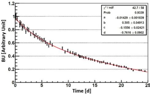
where the Burn-Up, BU, is the relative estimation over time,t, of the amount offissile material in the241Pu target used for the experiments (see for exampleFig. 1). The time evolution of the BU is carefully estimated by regularly measuring the overall ionic charge and kinetic energy distribution of mass 136, since it corresponds experimen-tally to an optimal count rate and mass separation. It is a mandatory normalization step since the amount offissile material is constantly decreasing over time due to the nuclear reactions consuming the 241Pu and the loss of material because of the harsh environmental conditions of the target [12]. The BU also takes into account the ion beamfluctuations over time as well as the incident neutron flux variations. Additional details on the procedure used for theBUmeasurement can be found in [13]. TheBUpoints arefitted in order to be extrapolated to the measurement times. No theoretical consideration is taken for the choice of the fit function due to the complexity of physical
phenomena governing the target behaviour. For the Exp.2 for example, theBUbehaviour is well reproduced by the sum of a polynomial of 1st order and an exponential function, as seen inFigure 1:
BUðtÞ ¼a⋅tþbþexpðc⋅tþdÞ: ð2Þ
Since the beam time is limited, the complete (Ek, q) distribution for each mass cannot be measured. The experimental method, refined over time [8,14,15], is to transform the sum over the ionic charge states into a division by the probability density function of the ionic charge states P(q), and the integral over the kinetic energies into a summation over bins of a constant step. Equation(1)becomes:
NqiðAÞ ¼
X
Ek
NðA;t;Ek;qiÞ PðqiÞ⋅BUðtÞ
: ð3Þ
One scan of the ionic charge states distribution at a constant kinetic energy is made for each mass and at least three scans of the kinetic energy distribution at different ionic charge states. Thanks to this, the ionic charge distribution P(q) can be estimated and at least three different values of the same N(A) are obtained: Nq1ðAÞ,
Nq2ðAÞandNq3ðAÞ, one for each measured kinetic energy distribution. To properly expressed Nq
iðAÞ, one should
take into account the existing correlation between the kinetic energy and ionic charge distributions [8,15]. To simplify the comparison proposed in this work, this step has been by-passed.
If the three estimations of the sameN(A) are compatible, the mean valueNðAÞtaking into account the experimental covariance matrix,C∈MnðℝÞ, is extracted by minimizing the generalizedx2[16]:
NðAÞ ¼ X
n;n
i;j
ðC1Þi;j
!1 Xn;n
i;j
ðC1Þi;j⋅NqjðAÞ
!
; ð4Þ
with a reduced variance:
VarNðAÞ¼ X n;n
i;j
ðC1Þi;j
!1
; ð5Þ
wherenis the number of energy scans for the massA. How C is obtained will be detailed in the Section 3.1. The compatibility is checked through a generalized x2 test taking into account the experimental covariances between theN(A)’s, such as thep-value is above 90% of confidence level:
x2ðNðAÞÞ ¼X n
i
Xn
j
ðNqiðAÞ NðAÞÞC 1
i;jðNqjðAÞ
NðAÞÞ: ð6Þ
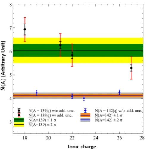
When this criterion is not met, an additional indepen-dent uncertainty,d, is incrementally added to the diagonal of the covariance matrixCof theN(A)’s, see equation(7), until a satisfyingx2is reached. This additional independent Fig. 1. The time evolution of the amount offissile material in the
uncertainty is accounting for theN(A)’s dispersion due to theflawed control of the instrument.
CiiðkÞ ¼Ciið0Þ þk⋅d; ð7Þ
where k is the number of increments. This process is illustrated inFigure 2.
As already specified in the introduction, two sets of experiments have been used in this analysis, thefirst one measured in May 2013, Exp.1, and the second one in November 2015, Exp.2. Since the experimental environment is different from one experience to the other (neutronflux, target, etc.,…) the two sets are considered as independent even though both are obtained on the LOHENGRIN mass spectrometer. The next step is thus to combine these two experiments to obtain the merged vectorNðAÞmgd(mgd stands for merged), by doing a relative normalization of one set to the other, relying on the value of theNðAÞ obtained for the 14 common masses, seeTable 1.
IfX andY are respectively the NðAÞvectors for the common masses of Exp.1 and Exp.2, then, to normalize Exp.1 with respect to Exp.2, one has to minimize the residual vectore:
e¼Yk⋅X: ð8Þ
The best estimator ofkis the normalization factorkof Exp.1 with respect to Exp.2, obtained through the generalized least square method, in its matrix form [17]:
k¼ ðXTV1XÞ1XTV1Y; ð9Þ
whereVis the combined covariance matrix for Exp.1 and Exp.2, taken to be V=VX+VY. Eventually, the mean values of the normalized set of the two experiments are extracted for the common masses in a similar way to equation(4).
The last step is the absolute normalization to obtain the yields,Y(A). Ideally, this normalization is done by taking Pi∈HNðAiÞmgd¼1, H being the masses of the heavy peak. This is true for pre-neutron yields when the contribution of ternaryfission is not taken into account. In our experiments, post-neutron yields from the masses 121 to 159 are obtained. The sum of the mass yields for A>159 represents 0.26% in JEFF-3.3 of the heavy peak and 0.03% for ENDF/B-VII.1. For the normalization step, a conservative uncertainty of 0.5% is taken, accounting for the absence of the very heavy masses, A>159 and the approximation that the sum over the heavy masses is equal to 1 for post-neutron yields.
However, since this document is only focused on high yields, the completeness of the Y(A) distribution for the heavy masses is not satisfyingly achieved. Nonetheless, in the scope of this document, the normalization will be done as previously explained, in order to discuss the impact of the absolute normalization.
Summary
The analysis path can be summarized in the following steps:
(1) sum over the kinetic energy distribution:
NðA;t;qiÞ ¼
P
EkNðA;t;Ek;qiÞ;
(2) determine theP(q) distribution and divide step (1) by P(qi):Nq
iðA;tÞ ¼ P
Ek
NðA;t;Ek;qiÞ
PðqiÞ ;
(3) evaluate the BU at t and divide step (2) by BU(t):
NqiðAÞ ¼ P
Ek
NðA;t;Ek;qiÞ
PðqiÞ⋅BUðtÞ;
(4) compute the mean value for each mass with eventual additional uncertainties:NðAÞ;
(5) normalize (relative normalization) and merge the two sets of experiments:NðAÞmgd;
(6) process the absolute normalization:Y(A).
3 Covariance matrices comparison
3.1 Differences between Monte-Carlo and analytical methods
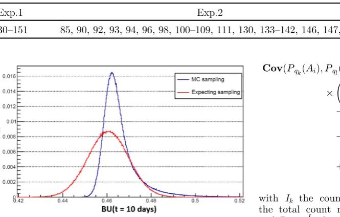
In the MC method, all count rates are sampled from a Poisson law. In order to assess BU(t), the fitted BU parameters are first decorrelated and then sampled from a Gaussian law with a unit standard deviation. The decorrelation is obtained through the equation(10)
[18]:
S¼V1=2
R R ð10Þ
with R is the fitted parameters,S the free parameters andVR is the covariance matrix of thefitted parameters. However, when theBUis computed from the sampling of the uncorrelated fit parameters, the probability density function obtained is no more a Gaussian distribution, see Figure 3. In the analytic method, when propagating uncertainties each parameter is supposed to have a Gaussian distribution, if it is not the case the biases of Fig. 2. EachNqiðAÞand their mean valueNðAÞfor the masses
this hypothesis should be controlled. This issue is under investigation. In order to still be able to compare the two analyses for the next steps, in the present work, the propagation of theBUuncertainties by the MC method is achieved analytically.
The covariance between N(A)’s, used in equation(4), can be decomposed between the covariances induced by the BUand the statistical covariances:
C¼CovðNqkðAiÞ;NqlðAjÞÞ ¼CovstatþCovBU; ð11Þ
Only covariance at the step (2) is computed through MC as expressed by equation (12), with m the MC event and Nq
kðAi;tÞ the arithmetic mean value of the NmqkðAi;tÞ’s.Covstat, the statistical part of the covariance
matrix is then defined as follows:
CovstatðNqkðAi;tÞ;NqlðAj;t
0ÞÞ
¼X
m
ðNmqkðAi;tÞ NqkðAi;tÞÞðN m qlðAj;t
0Þ N
qlðAj;t0ÞÞ;
ð12Þ
where t andt0 are respectively the times at which the mass Ai at the ionic charge state qk and the mass Aj at the ionic charge state ql have been measured. In the analytic case, equation (12) is written as equation
(13):
CovstatðNqkðAi;tÞ;NqlðAj;t
0ÞÞ
¼NqkðAi;tÞNqlðAj;t0Þ PqkðAiÞPqlðAjÞ
CovðPqkðAiÞ;PqlðAjÞÞ; ð13Þ
whereCovðPq
kðAiÞ;PqlðAjÞÞ is the covariance coming
from the ionic charge distribution. Therefore if Ai≠Aj, this term is null. Otherwise by propagating in a classical way the covariance, it is written:
CovðPqkðAiÞ;PqlðAiÞÞ ¼
P2kP
2
l I2kI
2
l
ðItotIkÞðItotIlÞCovðIk;IlÞ
ðItotIkÞIl
X
m≠l
CovðIk;ImÞ
ðItotIlÞIk
X
n≠k
CovðIn;IlÞ
þIkIl
X
m≠l
X
n≠k
CovðIm;InÞ
; ð14Þ
with Ik the count rates of the charge k, Itot=
P kIk the total count rate of the ionic charge distribution, andPk ¼ Ik
Itotthe normalized count rate. One has to note, since each measurement is independent, that only the diagonal of the covariance matrix of the count rate is not null.
TheBUcorrelation is taken into account analytically in both analyses through:
CovBUðNqkðAiÞ;NqlðAjÞÞ ¼
NqkðAiÞNqlðAjÞ BUikBUjl
CovðBUik;BUjlÞ; ð15Þ
with,
CovðBUik;BUjlÞ ¼
X m X n ∂BUik ∂rm ∂BUjl ∂rn
Covðrm;rnÞ;
ð16Þ
where {rk} are theBUparameters. As a consequence, for the analysis using MC, the following steps, (4–6), have to be computed analytically.
A final difference can be underlined. For independent parameters, the MC induces small correlations, even for pseudo-random numbers generated by different seeds. Since these correlations are low compared to the real experimental correlations, it is not an issue. It is worth noting that this MC numerical correlation artefact is dependent on the number of MC events. In this work, for 105events, the order of magnitude of this correlation artefact is 105.
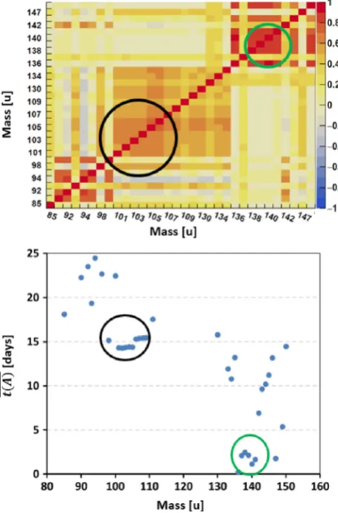
3.2 Step (3): impact of theBUon correlations
The BU is at this stage the only source of inter-masses correlations. To illustrate this, a mean experimental time
tðAÞhas been constructed for each mass.tðAÞis the mean time at which the massAis measured.
In Figure 4, one can see that masses having close experimental time have high correlation and vice versa. For example, the masses 100–109 (black circle) have been measured very closely in time, the same goes for the masses 138–141 (green circle). The correlations in these groups are very high, whereas inter groups correlations are close to 0.
Table 1. Set of masses measured in the two experiments and masses common to the two experiments.
Exp.1 Exp.2 Common masses
130–151 85, 90, 92, 93, 94, 96, 98, 100–109, 111, 130, 133–142, 146, 147, 149 130, 133–142, 146, 147, 149
The correlations obtained at this stage for the mix MC and analytic and the analytic methods are very similar, the highest absolute difference observed in the correlation matrix isDCorr¼0:0032 which represents a relative difference ofDCorrCorr ¼1:3%, seeFigure 5.
3.3 Step (4): impact of the additional dispersion uncertainties
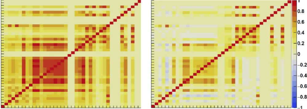
As it has just been explained, the correlation matrix is at this stage governed by theBU. The additional dispersion uncertainties introduced after equation(6), as independent uncertainties, wash away the initial structures. The weight of the common uncertainties coming from theBUis reduced. The impact of these additional uncertainties are shown inFigures 6 and7.
3.4 Step (5): impact of the relative normalization
The definition of the relative normalization factor k, in equation (9), is dependent on which experiment is the reference. Both the out-coming NðAÞmgd and the
associated correlation matrix will be affected, as it can be observed from Figures 8 and 9. Indeed, if Exp.1 is normalized with respect to Exp.2, the variance ofZ¼kX, the normalized vector of X, will be increased by the normalization, while the variance ofYremains constant. Ultimately, when the mean value for the common masses ofYandZis computed similarly to equation(4), taking into account the covariance matrices, NðAÞmgd depends on the experiment considered as the reference. As it can be seen in Figure 8, Exp.2 has initially smaller uncertainties. When it is the reference, the uncertainties after normalization are considerably smaller since they are monitored by Exp.2 uncertainties. On the contrary, mean values are barely sensitive to which reference is chosen.
In order to choose the reference, the cumulative eigenvalues of the correlation matrix is plotted inFigure 10. Afirst approach is to consider that a smooth increase of the cumulative eigenvalue is preferable. It means each mass brings a significant amount of information. The information is well spread between the different measurements and the correlation matrix is less structured. Considering this approach, the Exp.2 is taken as reference for the rest of this work. Work is in progress in order to construct an observable quantifying the quality of the information depending on the reference, similarly to the work presented in [19].
Fig. 5. The absolute difference in the correlation matrix between the two analyses at step (3).
Fig. 6. TheNðAÞdistribution with (in blue) and without (in red) the additional dispersion uncertainties (add. unc.) for Exp.2. Fig. 4. The correlations obtained in the analysis procedure for
Fig. 8. The relative difference on NðAÞmgd in black on the left axis, and on the uncertainty smgd in blue on the right axis, when the reference is Exp.1 or Exp.2. For the sake of the comparison, both sets of NðAÞmgd have been normalized to 1.
Fig. 7. The correlation matrix, for Exp.2, of theNðAÞwithout the additional dispersion uncertainties, on the left, and with, on the right.XandYlabels are identical toFigure 4(top).
A new analysis of the 2013 data is in progress and is expected to give results with lower uncertainties. In that case, it is expected that the choice of the reference has a reduced impact.
3.5 Step (6): impact of the absolute normalization
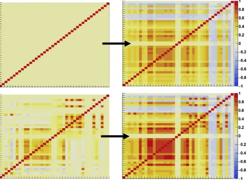
The impact on the Y(A) correlation matrix of the absolute normalization is illustrated in Figure 11. In
Figure 11, a diagonal correlation matrix is displayed (top left), while the analytic241Pu(nth,f) experimental
NðAÞmgd correlation matrix is shown (bottom left). On the right, the correlation matrices after the absolute normalization depending on which is the input correlation matrix. Thus, the effect of the absolute normalization step alone is shown on the top right of
Figure 11. TheY(A) correlation matrix (bottom right) is the combination of the effect of the absolute normalization alone and the experimental NðAÞmgd correlation matrix (bottom left).
The Y(A) correlation matrix structure is marked by the normalization procedure that creates a correlation background.
Fig. 10. The cumulative eigenvalues of the correlation matrix of theNðAÞfor the Exp.1 in blue and the Exp.2 in red.
Fig. 11. On top, the correlation matrix of the NðAÞmgd if inter-masses correlations are set to 0 (left) and its propagation through the absolute normalization (right). On the bottom, theNðAÞmgdanalytic correlation matrix (left) and its propagation
4 Conclusion and perspectives
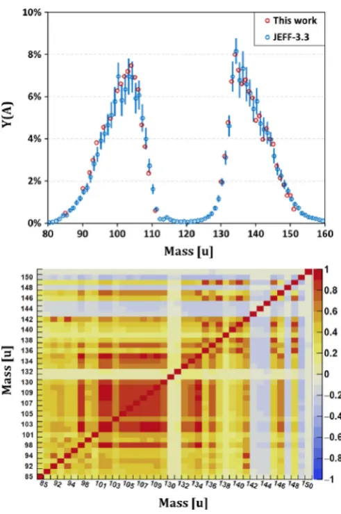
The experimentalY(A) obtained in this work is presented in Figure 12 and compared to JEFF-3.3. The precision achieved in this experimental work is much better than the JEFF-3.3 evaluation and significant discrepancies are observed, in particular in the light masses.
An effect not taken into account in this work is the correlation between the kinetic energy and ionic charge distributions. Since the ionic charge scan is made at a specific kinetic energy, Ek, this correlation has to be taken into account in order to properly estimateP(qi) in equation(3)
[20]. This is expected to significantly reduce the need of the additional dispersion uncertainties fromSection 3.3.
This work showed that both analyses give identical results for the estimation of the correlations matrix when the MC bias highlighted during theBUsampling step is by-passed. The BU sampling bias is under investigation in order to compare the MC and analytic methods on the full analysis scheme and not only on steps (1–3). For every
steps of the analysis scheme, the correlation matrices obtained by the two different analyses have been compared and no larger differences than the one observed at step (3) are seen, giving a strong confidence in our method. Mean values and uncertainties are also identical, validating both analyses. The structure of the correlation matrix is well understood, the importance of several steps in the construction of the correlation matrix have been empha-sized: theBUcreates strong positive correlations while the additional uncertainties due to the limits of the experi-mental methodflatten the correlation matrix. Finally the absolute normalization creates a correlation background.
The analyses have been compared without the correla-tion between the kinetic energy and ionic charge distribu-tions. In order tofinalize this work, a supplementary step where it is taken into account will be included to the analysis scheme. In addition, a re-analysis of the Exp.1 with updated tool and the construction of a reliable observable to rank the relative normalization possibilities are on going.
This work was supported by CEA, IN2P3 and“le défiNEEDS”. The authors are grateful for the support of the ILL and all the staff involved from CEA Cadarache and LPSC.
Author contribution statement
The analyses and their comparison as well as the writing of this manuscript have been conducted by S. Julien-Laferrière and A. Chebboubi.
This work was supported and supervised by G. Kessedjian and O. Sero, who participated to the elabora-tion of the method and the preparaelabora-tion of the manuscript.
References
1. H.G. Börner, F. Gönnenwein,The Neutron(World Scientific Publishing, Singapore, 2012)
2. N. Terranova et al., Ann. Nucl. Energy109, 469 (2017) 3. A. Plompen et al., Eur. Phys. J. A (to be submitted) 4. M.B. Chadwick et al., Nucl. Data Sheets112, 2887 (2011) 5. O. Serot et al., Nucl. Data Sheets119, 320 (2014) 6. P. Armbruster et al., Nucl. Instrum. Meth.139, 213 (1976) 7. H.R. Faust et al., ILL Internal Scientific Report 81FA45S, 1981 8. F. Martin, Ph.D. Thesis, Université de Grenoble, 2013 9. S. Julien-Laferriere et al., EPJ Web Conf.169, 00008 (2018) 10. H.R. Faust, Z. Bao, Nucl. Phys. A736, 55 (2004)
11. J.G. Heinrich, Report 6576, University of Pennsylvania, 2003 12. U. Köster et al., Nucl. Instrum. Methods A613, 363 (2010) 13. Y.K. Gupta et al., Phys. Rev. C96, (2017)
14. A. Bail, Ph.D. Thesis, Université Bordeaux I, 2009 15. A. Chebboubi, Ph.D. Thesis, Université de Grenoble-Alpes, 2015 16. M. Schmelling, Phys. Scr.51, 676 (1995)
17. A.C. Aitken, Proc. R. Soc. Edin. A55, 42 (1935)
18. A. Kessy, A. Lewin, K. Strimmer, Am. Stat. (2018), DOI: 10.1080/00031305.2016.1277159
19. B. Voirin et al., EPJ Nuclear Sci. Technol.4, 26 (2018) 20. F. Martin et al., Nucl. Data Sheets119, 328 (2014)
Cite this article as: Sylvain Julien-Laferrière, Abdelaziz Chebboubi, Grégoire Kessedjian, Olivier Serot, A study of the construction of the correlation matrix of241Pu(nth,f) isobaricfission yields, EPJ Nuclear Sci. Technol.4, 25 (2018)