A Numerical Study of Compressible Lid Driven Cavity Flow with a Moving Boundary

(1)

University of New Orleans University of New Orleans

ScholarWorks@UNO

University of New Orleans Theses and

Dissertations Dissertations and Theses

Spring 5-13-2016

A Numerical Study of Compressible Lid Driven Cavity Flow with a

Moving Boundary

Amer Hussain

UNIVERSITY OF NEW ORLEANS, [email protected]

Follow this and additional works at: https://scholarworks.uno.edu/td

Part of the Heat Transfer, Combustion Commons, and the Other Mechanical Engineering Commons

Recommended Citation Recommended Citation

Hussain, Amer, "A Numerical Study of Compressible Lid Driven Cavity Flow with a Moving Boundary" (2016). University of New Orleans Theses and Dissertations. 2155.

https://scholarworks.uno.edu/td/2155

This Thesis is protected by copyright and/or related rights. It has been brought to you by ScholarWorks@UNO with permission from the rights-holder(s). You are free to use this Thesis in any way that is permitted by the copyright and related rights legislation that applies to your use. For other uses you need to obtain permission from the rights-holder(s) directly, unless additional rights are indicated by a Creative Commons license in the record and/or on the work itself.

(2)

A Numerical Study of Compressible Lid Driven Cavity Flow with a

Moving Boundary

A Thesis

Submitted to the Graduate Faculty of the University of New Orleans in partial fulfillment of the requirements for the degree of

Master of Science in

Engineering Mechanical

by

Amer Hussain

B.Tech., Jawaharlal Nehru Technological University, 2014

(3)

ii

DEDICATION

To

My Parents

who brought me in this world and taught me never to lose hope and always try to the end without

expecting anything for earning an honest living

and

My Brother

who always encourages me to listen to my mind to do things as I think is good and always keeps

(4)

iii

ACKNOWLEDGMENT

First of all, I would like to express my sincere gratitude to my advisor, Dr. Kazim M

Akyuzlu for the continuous support of my Master’s study and research, for his patience,

motivation, enthusiasm, and immense knowledge. I am thankful for his guidance on fostering my

professional problem-analyzing, problem-solving, and reporting skills. His advice helped me a

lot to complete this work.

Besides my advisor, I would like to thank the rest of my thesis committee; Dr. Ting Wang

and Dr. Martin J Guillot for their encouragement and insightful comments.

I thank my fellow lab mates M Shafiqur Rahman, Anvesh Nallaballi, Mine Kaya, Jose E.

Rubio, Seda Aslan, and Pratik Sarker at the University of New Orleans for the stimulating

discussions, sleepless nights we worked together before deadlines, and for all the fun we have

had in the last two years.

Last but not the least, I would like to thank my family, my father Hussain Rafi Ullah and

my mother Shameem Akhtar for bringing forth me in this world and supporting me unanimously

(5)

iv

ABSTRACT

A two-dimensional (2-D), mathematical model is adopted to investigate the development

of circulation patterns for compressible, laminar, and shear driven flow inside a rectangular

cavity. The bottom of the cavity is free to move at a specified speed and the aspect ratio of the

cavity is changed from 1.0 to 1.5. The vertical sides and the bottom of the cavity are assumed

insulated. The cavity is filled with a compressible fluid with Prandtl number, Pr =1. The

governing equations are solved numerically using the commercial Computational Fluid

Dynamics (CFD) package ANSYS FLUENT 2015 and compared with the results for the

primitive variables of the problem obtained using in house CFD code based on Coupled

Modified Strongly Implicit Procedure (CMSIP). The simulations are carried out for the unsteady,

lid driven cavity flow problem with moving boundary (bottom) for different Reynolds number,

Mach numbers, bottom velocities and high initial pressure and temperature.

Keywords: Lid Driven Cavity Flow, Compressible, Unsteady, Laminar, CFD models, Moving

(6)

v

NOMENCLATURE

Symbols

AR cp

H k L M Pr p R Re T t u v x y

Aspect Ratio, H/L

Specific Heat

Height of the cavity

Thermal conductivity

Width of the cavity

Mach number

Prandtl number

Pressure

Gas Constant

Reynolds number

Temperature

Time

Velocity in x direction

Velocity in y direction

Horizontal distance

Vertical distance

Greek Symbols

γ Isentropic constant

µ Viscosity

ρ Density

𝜙 Viscous dissipation

𝜉 Transformed x coordinate

𝜎 Transformed y coordinate

Superscripts

(10)

ix

List of Figures

Figure 1 – Schematic of a square cavity with a moving bottom

Figure 2 – Mesh of the computational domain

Figure 3 – Overview of pressure-based coupled algorithm

Figure 4 – Computational Molecule for the Elements of A Matrix

Figure 5 – Computational Mesh for the Transformed () Domain

Figure 6 – Computational mesh of the domain

Figure 7 – u velocity contour for Re = 400

Figure 8 – Vectors of velocity magnitude for Re=400

Figure 9 – Streamlines of velocity magnitude for Re=400

Figure 10 – Contour plot of pressure for Re=400

Figure 11 – Contour plot of temperature for Re=400

Figure 12 – u velocity distribution along vertical centerline for Re=400

Figure 13 – v velocity distribution along horizontal centerline for Re=400

Figure 14 –Distribution of Horizontal Velocity (𝑢̅) along Centerline Vertical Distance for

Re = 100 and AR 1.0.

Re = 400 and AR 1.0

Re = 1000 and AR 1.0

Figure 17 –Distribution VerticalVelocity (𝑣̅) along Centerline Horizontal Distance for

(11)

x

Figure 18 –Distribution of VerticalVelocity (𝑣̅) along Centerline Horizontal Distance for

Re = 400 and A.R 1.0

Re = 1000 and A.R 1.0

Re = 400 and A.R 1.0 for different mesh sizes

Figure 21 –Distribution of Vertical Velocity (𝑣̅) along Centerline Horizontal Distance for

Re = 400 and A.R 1.0 for different mesh sizes.

Re = 100 and A.R 1.0

Re = 400 and A.R 1.0

Re = 1000 and A.R 1.0

Re = 100 and A.R 1.0

Re = 400 and A.R 1.0

Figure 27 – Distribution of Vertical Velocity (𝑣̅) along Centerline Horizontal Distance for

Re = 1000 and A.R 1.0

Figure 28 – Pressure contour plot for Re = 100 (FLUENT)

(12)

xi

Figure 31 – Pressure contour plot for Re = 400 (CMSIP)

Figure 33 – Pressure contour plot for Re = 400 (CMSIP)

Figure 34 – Temperature contour plot for Re = 100 (FLUENT)

Figure 35 – Temperature contour plot for Re = 1000 (CMSIP)

Figure 40 – Schematic of the infinite rectangular cavity of AR 3.0

Figure 41 – Dynamic Layering

Figure 42 – Computational mesh of the domain before moving of the bottom boundary (A.R 3.0)

Figure 43– Deforming of mesh using Spring-Based Smoothing technique

Figure 44 – 𝑣̅ velocity histogram for the motion of bottom boundary at at node at

𝑥̅ = 0.0, 𝑦̅ = 0.0 for different mesh motion studies.

Figure 45 – Computational mesh of the domain after moving of the bottom boundary using

layering technique (AR 3.0)

Figure 46 – Computational mesh of the domain after moving of the bottom boundary using

Spring-Based technique (AR 3.0)

Figure 47 – Computational mesh of the domain after moving of the bottom boundary using user-

defined technique (A.R 1.5)

(13)

xii

(a. using Layering, b. Using Spring-Based and c. Using UDF)

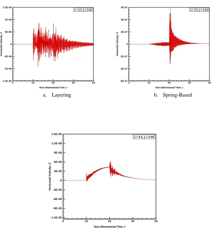
Figure 49– 𝑣̅ velocity histogram at node at 𝑥̅ = 0.5, 𝑦̅ = 0.68 for different mesh motion studies.

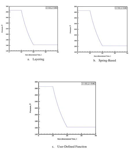
Figure 50 – 𝑃̅ pressure histogram at node at 𝑥̅ = 0.5, 𝑦̅ = 0.68 for different mesh motion studies

Figure 51 – 𝑇̅ Temperature histogram at node at 𝑥̅ = 0.5, 𝑦̅ = 0.68 for different mesh motion

studies. (a. using Layering, b. Using Spring-Based and c. Using UDF)

Figure 52 – 𝜌̅ Density histogram at node at 𝑥̅ = 0.5, 𝑦̅ = 0.68 for different mesh motion studies

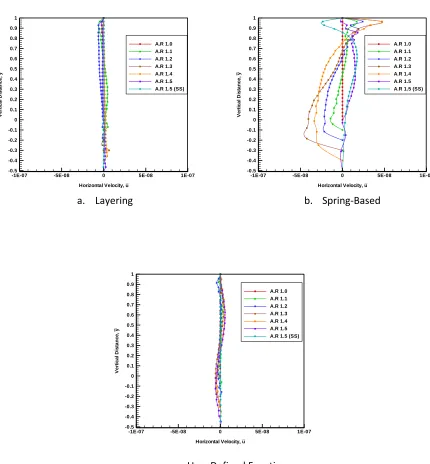
Figure 53 – u̅ velocity distribution along centerline vertical distance ( y̅ = 0.0 to 1. 0) at 𝑥̅ = 0.5

for different mesh motion studies. (a. using Layering, b. Using Spring-Based and

c. Using UDF)

Figure 54 – v̅ velocity distribution along centerline vertical distance ( x̅ = 1.0 to 2. 0) at 𝑥̅ = 0.5

for different mesh motion studies (a. using Layering, b. Using Spring-Based and

c. Using UDF)

Figure 55 – Comparison of u̅ velocity distribution along centerline vertical distance for

( y̅ = 0.0 to 1. 0) at 𝑥̅ = 0.5 and time t̅ = 12 for different mesh motion studies and AR 1.1

Figure 56 – Comparison of u̅ velocity distribution along centerline vertical distance for

( y̅ = 0.0 to 1. 0) at 𝑥̅ = 0.5 and time t̅ = 14 for different mesh motion studies and AR 1.2

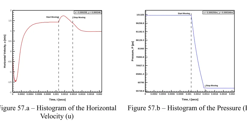
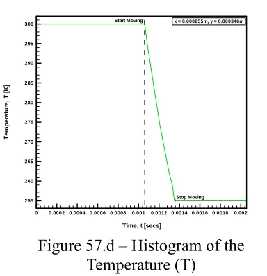
Figure 57 (a – d) – Histogram of the Horizontal Velocity (u)at x = 0.000255, y = 0.000346

before, during, and After the Motion of the Bottom Boundary of the Cavity for AR = 1.5

and Re = 400.

(14)

xiii

Re = 400

Figure 59 – Vertical Velocity (v) Distribution along Centerline Vertical Distance (x) for Re = 400

Figure 60 – Vector plot of velocity magnitude at t = 0 sec and AR 1.0

Figure 61 – Vector plot of velocity magnitude at t = 0.0000035 sec and AR 1.0

Figure 74 – Streamline plot of velocity magnitude at t = 0 sec and AR 1.0

Figure 75 – Streamline plot of velocity magnitude at t = 0.0000035 sec and AR 1.0

(15)

xiv

Figure 88 – Pressure Contour at t = 0.00106 sec and AR 1.0

Figure 89 – Temperature Contour at t = 0.00106 sec and AR 1.0

(16)

xv

Figure 102 - 𝑢̅ velocity comparison at 𝑡̅ = 35 and AR 1.0 for different time increments Figure 103 - 𝑢̅ velocity comparison at 𝑡̅ = 46 and AR 1.5 for different time increments Figure 104 - 𝑣̅ velocity comparison at 𝑡̅ = 35 and AR 1.0 for different time increments Figure 105 - 𝑣̅ velocity comparison at 𝑡̅ = 46 and AR 1.5 for different time increments Figure 106 - 𝑢̅ velocity comparison at 𝑡̅ = 35 and AR 1.0 for different grid sizes Figure 107 - 𝑢̅ velocity comparison at 𝑡̅ = 46 and AR 1.5 for different grid sizes Figure 108 - 𝑣̅ velocity comparison at 𝑡̅ = 35 and AR 1.0 for different grid sizes Figure 109 - 𝑣̅ velocity comparison at 𝑡̅ = 46 and AR 1.5 for different grid sizes

Figure 110– Comparison of 𝑢̅ velocity between CMSIP and FLUENT at 𝑡̅ = 35 and AR 1.0

Figure 111– Comparison of 𝑢̅ velocity between CMSIP and FLUENT at 𝑡̅ = 38 and AR 1.1

Figure 112– comparison of 𝑢̅ velocity between CMSIP and FLUENT at 𝑡̅ = 46 and AR 1.5

Figure 113 – comparison of 𝑢̅ velocity between CMSIP and FLUENT at t̅ = 70 and AR 1.5

Figure 114 – Comparison of 𝑣̅ velocity between CMSIP and FLUENT at 𝑡̅ = 35 and AR 1.0

Figure 115 – Comparison of 𝑣̅ velocity between CMSIP and FLUENT at 𝑡̅ = 38 and AR 1.1

Figure 116 – comparison of 𝑣̅ velocity between CMSIP and FLUENT at 𝑡̅ = 46 and AR 1.5

Figure 117 – comparison of 𝑣̅ velocity between CMSIP and FLUENT at t̅ = 70 and AR 1.5

Figure 118 – Streamline plot for velocity magnitude at AR 1.0 (FLUENT)

Figure 119 – Streamline plot for velocity magnitude at AR 1.0 (CMSIP)

Figure 121 – Streamline plot for velocity magnitude at AR 1.1 (CMSIP)

(17)

xvi

Figure 124 – Streamline plot for velocity magnitude at AR 1.5 Steady State (FLUENT)

Figure 125 – Streamline plot for velocity magnitude at AR 1.5 Steady State (CMSIP)

Figure 126 – Bottom velocity profiles

Figure 127 - 𝑢̅ velocity histogram at node 𝑥̅ = 0.5, 𝑦̅ = 0.68

Figure 128 – Streamline plot of velocity magnitude at AR 1.3 with 𝑣̅_𝑏 = −0.025

Figure 131 - Comparison of the 𝑢̅ velocities for different bottom boundary velocities

at 𝑡̅ = 42, 𝐴𝑅 1.3

Figure 132 - Comparison of the 𝑣̅ velocities for different bottom boundary velocities

at 𝑡̅ = 42, 𝐴𝑅 1.3

Figure 133 – Streamline plot of velocity magnitude at AR 1.0 for Re 100

Figure 139 - Comparison of the 𝑢̅ velocities for different Re number 𝑡̅ = 36, 𝐴𝑅 1.0

Figure 140 - Comparison of the 𝑢̅ velocities for different Re number 𝑡̅ = 46, 𝐴𝑅 1.5

(18)

xvii

Figure 142 - Comparison of the 𝑣̅ velocities for different Re number 𝑡̅ = 46, 𝐴𝑅 1.5

Figure 143 - Comparison of the 𝑣̅ velocities for different M number 𝑡̅ = 36, 𝐴𝑅 1.0

Figure 144 - Comparison of the 𝑣̅ velocities for different M number 𝑡̅ = 46, 𝐴𝑅 1.5

Figure 145 – Streamline plot of velocity magnitude at AR 1.0 for P = 100kpa,T = 300K

Figure 146 – Streamline plot of velocity magnitude at AR 1.0 for for P = 100kpa,

T = 700K

Figure 147 – Streamline plot of velocity magnitude at AR 1.0 for for P = 506kpa,

T = 300K

Figure 148 – Streamline plot of velocity magnitude at AR 1.5 for for P = 100kpa,T = 300K

(19)

xviii

List of Table

Table 1 – Fluent solver settings

Table 2 – Common simulation Parameters for Lid Driven Cavity flow for Re = 400 by FLUENT

Table 3 – Results for Lid Driven Cavity flow for Re = 400 by FLUENT

Table 4 – Comparison of the results for u velocities obtained from the benchmark, CMSIP, and

FLUENT at different values of Re

Table 5 – Comparison of the results for v velocities obtained from the benchmark, CMSIP, and

Table 6 –Results for grid independence study for steady state driven cavity flow

Table 7 –Results for different Reynolds number Study for Steady

State Driven Cavity Flow

Table 8 – Simulation parameters for infinite rectangular cavity

Table 9 – Comparison of 𝑢̅ and 𝑣̅ velocities for different time increments

Table 10.a – Comparison of 𝑢̅ velocities for different grid sizes at A.R 1.0 and 1.5

Table 10.b - Comparison of 𝑣̅ velocities for different grid sizes at A.R 1.0 and 1.5

Table 11 – Comparison of distribution of 𝑢̅ velocity at AR 1.0 and 1.1 for FLUENT and CMSIP.

Table 12 – Comparison of distribution of 𝑢̅ velocity at AR 1.5 and 1.5 (steady state) for FLUENT

and CMSIP.

Table 13 – Comparison of distribution of 𝑣̅ velocity at AR 1.0 and 1.1 for FLUENT and CMSIP.

Table 14 – Comparison of distribution of 𝑣̅ velocity at AR 1.5 and 1.5 (steady state) for FLUENT

and CMSIP.

(20)

xix

at 𝑡̅ = 42, 𝐴𝑅 1.3

Table 16 – Comparison of the 𝑣̅ velocities for different bottom boundary velocities

at 𝑡̅ = 42, 𝐴𝑅 1.3

Table 17 – Comparison of the results (maximum velocities) of the unsteady lid driven cavity flow

with different Re = 100, 400 and 1000 at different aspect ratios

Table 18 – Comparison of the results (maximum velocities) of the unsteady lid driven cavity flow

with different Re = 100, 400 and 1000 at different aspect ratios

Table 19– Comparison of the 𝑢̅ velocities for Ma = 0.01, 0.03 and 0.05 at different aspect ratios

Table 20 – Comparison of the 𝑣̅ velocities for Ma = 0.01, 0.03 and 0.05 at different aspect ratios

(21)

1

1.

Introduction

Lid Driven cavity flow has been used extensively in the past as a benchmark case for the

study of computational methods to solve Navier-Stokes equations. In this problem the side and

bottom walls (boundaries) surrounding the cavity are fixed but the upper surface (lid) of the

cavity is moved at a uniform velocity. Many investigators [1-8] have solved this problem

assuming an incompressible fluid at low Mach numbers inside a cavity. This incompressible

flow version of the driven cavity problem seems to be the benchmark case which is widely used

by other investigators who study compressible flow inside cavities or channels. Some researchers

[9] have used this classical problem to benchmark their solutions to unsteady compressible

Navier-Stokes equations for low and high Mach number laminar flows. (Experimental data is

also available for this problem. See references [10-12].)

Other benchmarking cases include flow in a channel, flow though an expansion, and external

flows over various types of solid surfaces. All of these cases, including the driven cavity

problem, represent examples of fixed boundary problems where steady state solutions to

incompressible (and compressible) Navier-Stokes equations are of concern. No attempt has been

made yet to establish a benchmark case to study various solution techniques for moving

boundary problems.

So far there is no available benchmarking solutions to unsteady, compressible Navier-Stokes

equations where the flow domain is not enclosed by fixed boundaries. An example of such type

of problems is the case of natural convection inside the ullage of a cryogenic storage tank where

(22)

2

moving boundary problems is the flow of combustion gases inside the combustion chamber of a

hybrid rocket motor where the chamber boundaries move (enlarge) with the continuous ablation

of the solid fuel surface [14]. Both of these problems require the solution of the unsteady,

compressible Navier-Stokes equations and the coupled energy equation to predict, accurately, the

velocity field as well as the temperature and pressure distributions inside the flow domain.

An attempt has been made to simulate a lid driven cavity flow at aspect ratio 1.0 with a

moving boundary using Coupled Modified Strongly implicit Method (CMSIP) by Akyuzlu et. al

[15], where the bottom of the cavity is assumed to move at a constant speed until the aspect ratio

of 1.5 is reached.

Here a commercial CFD package ANSYS FLUENT is used to simulate the similar case [15]

and compare the results, to illustrate the accuracy of the simulation for better characterizations of

(23)

3

2.

Literature Survey

Assuming incompressible flow inside the cavity, numerous investigations have been done

[1−7] with low M and variable Re values to solve the problem. This study of incompressible

flow has been the benchmark for years with widespread applications for the researchers

including the study of channel flows, cavity flows, low and high Mach number laminar

compressible flows [8−10]. Ghia et al. used the vorticity-stream function formulation of the

two-dimensional incompressible Navier- Stokes equations to study the effectiveness of the coupled

strongly implicit multigrid (CSI-MG) method in the determination of high-Re fine-mesh flow

solutions. This work has been considered as a benchmark research to be studied by many fellow

researchers in the last few decades [2−8].

Chen and Pletcher [9] used the classical problem to benchmark their solutions to unsteady

compressible Navier-Stokes equations for low and high Mach number laminar flows. Other

benchmarking cases include flow in a channel, flow through an expansion, and external flows

over various types of solid surfaces. All of these cases, including the driven cavity problem,

represent examples of fixed boundary problems where steady state solutions to incompressible

(and compressible) Navier-Stokes equations are of concern. There is a need for benchmarking

solutions to unsteady, compressible Navier-Stokes equations where the flow domain is not

enclosed by fixed boundaries. An example of such type of problems is the case of natural

convection inside the ullage of a cryogenic storage tank where the ullage volume increases with

the discharge of the liquid propellant [13]. Another example of moving boundary problems is the

flow of combustion gases inside the combustion chamber of a hybrid rocket motor where the

chamber boundaries move (enlarge) with the continuous ablation of the solid fuel surface [14].

(24)

4

equations and the coupled energy equation to predict, accurately, the velocity field as well as the

temperature and pressure distributions inside the flow domain.

A study with moving bottom boundary for compressible flow has also been conducted by

Akyuzlu et al, [11] where the change of aspect ratio of the driven cavity due to the moving

bottom wall has been analyzed. In that study, the set of algebraic equations corresponding to the

problem have been solved by using the Coupled Modified Strongly Implicit Procedure (CMSIP)

for the unknown primitive variables. Again, other mentionable attempts relating to this field are

the numerical study of natural convection of compressible fluid inside an enclosed cavity [12],

(25)

5

3.

Description of The Physical Model

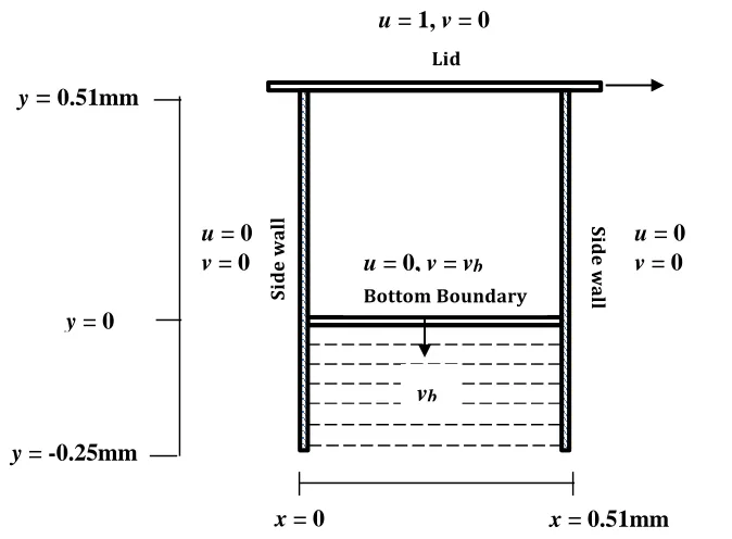
In the present study, a square cavity of aspect ratio 1.0 filled with compressible fluid at Pr = 1.0 is used as working fluid at standard temperature and pressure (STP). The top, left, right, and

bottom walls of the cavity are considered to be adiabatic walls with no slip condition. Initially,

everything is stationary inside the square cavity. The flow becomes steady at time (t1), then the

bottom boundary is moved with a constant velocity (vb) in negative y direction which stops at

time (t2) when the square cavity reaches the aspect ratio of 1.5 and becomes steady again at time

(t3). Evaluating the values M and Re, the flow inside the cavity can be categorized as laminar and subsonic. The physical model of the square cavity is shown in Figure 1.

Figure 1 – Schematic of a square cavity with a moving bottom

y = 0.51mm

y = 0

y = -0.25mm

x = 0 x = 0.51mm

u = 1, v = 0

u = 0, v = vb

u = 0

v = 0

u = 0

v = 0

𝛛𝐓

𝛛𝐱 _v

b

𝐋𝐢𝐝

𝐁𝐨𝐭𝐭𝐨𝐦 𝐁𝐨𝐮𝐧𝐝𝐚𝐫𝐲

𝐒𝐢

𝐝𝐞

𝐰

𝐚𝐥

𝐥

𝐒𝐢

𝐝𝐞

𝐰

𝐚𝐥

(26)

6

No slip boundary conditions are assumed on the walls of the cavity and also considered to be

impermeable. There is no heat transfer through the walls since they are adiabatic. With constant

(27)

7

4.

Description of a Mathematical Model

The mathematical formulation of the driven cavity including the conservation equations

together with the initial and boundary conditions in second order accurate in time models is

given in this chapter. The dimensional governing equations used is derived from the respective

vector form of continuity, momentum, and energy equations (refer to Appendix I). The initial

and boundary conditions are then applied to well pose the mathematical formulation.

4.1 2-D Mathematical Model (FLUENT)

4.1.1 Assumption of 2-D Mathematical Model

The following assumptions were made for the present study.

1. The physical domain is Two-dimensional and the equations are in Cartesian Coordinates.

2. The working fluid forms a continuum.

3. The flow is subsonic, unsteady, laminar, and viscous.

4. The working fluid is compressible with Pr = 1 (the density of the fluid is a function of

temperature and pressure) and can be treated as an ideal gas.

5. The working fluid behaves like a Newtonian fluid with stokes assumptions.

6. The kinetic and potential energy terms in the energy equations are very small and can be

neglected except viscous dissipation term.

7. Radiation heat transfer is ignored.

8. There are no internal heat sources.

9. The physical and transport properties of the fluid are assumed to be constant

(28)

8

4.1.2 Mathematical Formulation for 2-D Model

i. Governing Differential Equations

The conservation equations for 2-D, unsteady, viscous, compressible, subsonic, and

laminar flow can be written in terms of primitive variables ρ, u, T, and P as follows:

For 2-D Cartesian, unsteady, compressible fluid, the conservative form of these equations are

given as follows:

The continuity equation is given by:

0 ) ( ) (          v y u x

t



(4.1)

The momentum equation in the x-direction is given by:

                                        ) ( ) 2 ( 3 2 ) ( ) ( ) ( 2 x v y u y y v x u x x p uv y u x u t      (4.2)

The momentum equation in the y-direction (normal to fuel surface) is given by:

                                           ) 2 ( 3 2 ) ( ) ( ) ( ) ( 2 x u y v y x v y u x y p y p v y v u x v t      (4.3)

The energy equation is given by:





] ) ( 3 2 ) ( ) ( 2 ) ( 2 [ ) ( ) ( ) ( ) ( ) ( 2 2 2 2 y v x u y u x v x v x u y T k y x T k x T v c y T u c x T R c

t p p p

(29)

9

The equation of state is given by

p RT (4.5)

ii. Initial Conditions

1 0 , 1 0 0 , 1 0 , 1 0 0 , 0 , 0                     y x and t at P P T T y x and t at v u o i o i o i  

iii. Boundary conditions

Therefore, the governing equations are Non-Linear, second order and coupled.

4.2 2-D Mathematical model (CMSIP)

4.2.1 Assumption of 2-D Mathematical Model

The following assumptions were made for this mathematical model.

1. The physical domain is Two-dimensional and the equations are in Cartesian Coordinates.

2. The working fluid forms a continuum.

3. The flow is subsonic, unsteady, laminar, and viscous.

(30)

10

4. The working fluid is compressible with Pr = 1 (the density of the fluid is a function of

temperature and pressure) and can be treated as an ideal gas.

5. The working fluid behaves like a Newtonian fluid with stokes assumptions.

6. The kinetic and potential energy changes of the fluid, viscous dissipation, and the work

done by the pressure changes are small. (The terms representing these changes are ignored

in the energy equation.) These assumptions are valid for low Mach number flows (M< 0.1).

7. There are no internal heat sources.

8. The physical and transport properties of the fluid are assumed to be constant

9. No effect of gravity is assumed on the enclosed fluid.

4.2.2 Mathematical Formulation for 2-D Model

i. Governing Differential Equations

The non-dimensional conservation equations for a two-dimensional, unsteady, viscous,

compressible flow for low Mach numbers can be written in terms of non-dimensional form of the

primitive variables 𝑢̅, 𝑣,̅ 𝑝̅ and 𝑇̅ by replacing density by pressure and temperature using the

equation of state ( ρ = p/RT ) for ideal gases as follows: The continuity equation is given by:

0                            T v p y T u p x T p

t (4.6)

The momentum equation in the x-direction is given by:

 

2 0

(31)

11

The momentum equation in the y-direction is given by:

 

2 0

3 2 2                                                                       y v x u y e R R x v y u x e R R p R y T v p y T v u p x T v p t   (4.8)

The energy equation is given by:

















_0

                              y T y r P e R c R x T x r P e R c R c v p y c u p x R C p t p p p p p   (4.9)

ii. Initial conditions

The governing equations of the present problem are solved for the initial conditions at

which the fluid inside the cavity is assumed stagnant and isothermal (at atmospheric conditions).

The initial pressure distribution inside the cavity is determined from solution of the hydrostatic

equation.

iii. Boundary conditions

The mathematical formulation is closed by the following boundary conditions for time t > 0:

(32)

12

The non-dimensional variables used in the above formulation are defined as follows:

ref ref ref ref ref ref p ref ref p p ref ref ref ref ref ref ref ref ref ref ref ref ref μ L u ρ e R , T R γ u M , k μ c r P , /T u c c , /T u R R , μ μ μ , ρ ρ ρ , T T T , u ρ p p , u v v , u u u , L y y , L x x , /u L t t               2 2 2

(33)

13

5.

Numerical Formulation and Solution Procedures

In this study, a 2-D model is simulated using ANSYS FLUENT 2015 under the given boundary

conditions. The working fluid in the cavity is at STP with M = 0.05 and Pr = 1.

5.1The Pressure-Based Coupled Algorithm

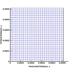
5.1.1 Discretization

ANSYS FLUENT uses a control-volume-based technique to convert the governing equations

to algebraic equations that can be solved numerically by integrating the governing equations

about each control volume, yielding discrete equations that conserve each quantity on a

control-volume basis. The governing equations are discretized for the mesh (29 x 29) as shown in the

figure 2.

Figure 2 – Mesh of the computational domain

Horizontal Distance, x

V

e

rt

ic

a

l

D

is

ta

n

c

e

,

y

0 0.0001 0.0002 0.0003 0.0004 0.0005 0

(34)

14

5.1.2 Solutions Technique

The discretized governing equations are solved using Pressure-Based solver [17] as the

governing equations are non-linear and coupled. Therefore, the solution is carried out iteratively

in order to obtain a converged numerical solution. The Pressure-based solver uses a solution

algorithm which can solve the non-linear equations. There are four algorithms available in this

technique namely Semi-Implicit Method for Pressure-Linked Equations (SIMPLE),

SIMPLE-Consistent (SIMPLEC), Pressure Implicit with Splitting of Operators (PISO), and Coupled. In

this Study “Coupled” algorithm was used since the momentum and continuity equations are

solved in a closely coupled manner except energy equation which is solved in a decoupled

fashion and therefore, the rate of solution convergence significantly improves when compared to

the other techniques. Second-order upwind scheme is used for the spatial discretization of

governing equation while the Second-order implicit scheme is used for transient formulation.

With the Pressure-Based Coupled Algorithm, each iteration consists of the steps illustrated in

figure 2. The algorithm is outlined below:

1. Update fluid properties (e.g., density, viscosity, specific heat) based on the current

solution.

2. Solve a coupled system of equations comprising the momentum and pressure-based

continuity equation. The remaining equations are solved in decoupled fashion.

3. Update mass fluxes, pressure and the velocity field.

4. Solver energy equation.

5. Check for the convergence of the equations.

(35)

15

(36)

16

The solver settings used in ANSYS FLUENT are mentioned in table 1

Table 1 – Fluent solver settings

CFD SOLVER SETTINGS

Description Settings

Problem Setup – Solver Pressure Based

Viscous Laminar

Pressure-Velocity Coupling Coupled

Gradient Discretization Green Gauss Cell Based

Pressure Discretization Second Order upwind

Density Discretization Second Order upwind

Momentum Discretization Second Order upwind

Energy Second Order upwind

Transient formulation Second Order upwind

Residual Criteria 1E-15

5.2 Coupled Modified Strongly Implicit Procedure (CMSIP)

A modified version of the Coupled Strongly Implicit Procedure (CSIP), developed by

Akyuzlu et al. [15] and details of this procedure the reader should refer to Appendix [II]

It is assumed that the changes in kinetic and potential energy of the fluid, viscous

dissipation, and the work done by the pressure changes are small. The density in the governing

(37)

17

5.2.1 Transformation

The 𝑥̅ and 𝑦̅ oordinate system used in development of the conservations equations,

(Equations 4.6 to 4.9), are transformed to the rigid (non-moving) coordinate 𝜉̅ and σ̅ system as

follows [15]:

H y





(5.1)

where H _{is defined as (}_h_and_r_{are normalized using}_L_ref₎

 

x,t

r h

H  

(5.2)

and

x





(5.3)

Based on the transformation given above the first order derivatives of any variable are given by:

) ( t ) ( t ) (

t 



     

  



(5.4)

where

r H t

) t , x ( r H t

t 

 



 

      

(5.5)

and

) ( x ) ( ) (

x 



 

    

  



(5.6)

where

x ) t , x ( r H x

x 

    

  



(38)

18

and

) ( y ) (

y 

 

    



(5.8)

where

H 1 y

y  

 



(5.9)

The second order partial derivative with respect to x is given by:

)] ( ) x

) t , x ( r H ( [ ))

( ( ))

( x (

x 

  

 

 

  

  

 

  

 



(5.10)

The second order partial derivative with respect to y is given by:

) ) ( H

1 ( )

) ( y (

y  2 

 

  

 



(5.11)

The final version of the transformed form of the non-dimensional conservation equations is

given in the Appendix [III].

5.2.2 Discretization

First, the governing differential equations (in non-dimensionalized and transformed form)

are discretized using first order forward differencing for the time derivative terms, central

differencing (second order accuracy) for all spatial derivatives (that is convective, viscous, and

thermal diffusion terms) and pressure terms. Central differencing of flux (momentum and

(39)

19

flux quantities at each opposing side of the computational cell. See [15] for details of the

discretization.

5.2.3 Linearization

The discretized non-dimensional conservation equations are linearized by Newton’s linearization

method. For example, the nonlinear term (P/T) in the continuity equation is linearized for the

(n+1)th time (where n indicates the discretized time level and k indicates the iteration index) as follows:







k 1 k



1 k k 1 k 1 k k 1 k T T T ) T p ( p p p ) T p ( ) T p ( ) T p (               (5.12)

After linearization, the conservation equations are put into following form for any nodal

point (i, j) of the computational domain [15] :

j , i 1 j , 1 i 2 j , i 1 j , i 1 j , i 1 j , 1 i 8 j , i j , 1 i 3 j , i j , i 9 j , i j , 1 i 7 j , i 1 j , 1 i 4 j , i 1 j , i 5 j , i 1 j , 1 i 6 j , i

b

x

A

x

A

x

A

x

A

x

A

x

A

x

A

x

A

x

A





            (5.13)

Similar equations are generated for the rest of the inner nodal points of the computational

domain. The resulting set of algebraic equations (as many as the number of inner nodes) is then

put into block matrix form [15]

 

A

x



b

(5.14)

Where [A] is the coefficient matrix with a 4x4 block in each element, x is the unknown vector,

(40)

20

Figure 4 – Computational Molecule for the Elements of A Matrix

Figure 5 – Computational Mesh for the Transformed () Domain

Horizontal Distance,

V

e

rt

ic

a

l

D

is

ta

n

c

e

,

0 0.25 0.5 0.75 1

0

0.1

0.2

0.3

0.4

0.5

0.6

0.7

0.8

0.9

1









j+1

j

j-1

(41)

21

6. Steady State Lid Driven Cavity Flow – Results for Benchmark Case

Study

In this study, numerical studies have been carried out to obtain the steady state solution of

compressible lid driven cavity flow for various Reynolds number (100, 400, and 1000). The results

obtained using FLUENT and CMSIP are validated by comparing with the benchmark case [1] by

Ghia et.al [1] which solves for incompressible flow using vorticity equation and is shown in

Figures through 6. Also a grid independence study is done to establish the accuracy of the solution.

6.1 Results for Steady State Lid Driven Cavity Flow Using Fluent.

In this study a compressible fluid at Ma = 0.05 and Pr = 1 is enclosed in a square cavity

of aspect ratio 1.0 (L = H = 0.00051m in this case) at STP is assumed. The lid of the cavity is

given a constant velocity at Re = 400 (17.3205m/ in this case) and the steady state solution using

grid size of 39 x 39 obtained from FLUENT is shown in Figure 6.1. The parameters used and

results for maximum u and v velocities are quantified in Table 2.

Table 2 – Common simulation Parameters for Lid Driven Cavity flow for Re = 400 by FLUENT

Simulation Parameters

Parameter Unit Value

Length, L [m] 0.00051

Height, H [m] 0.00051

Lid Velocity, 𝑢_𝑙𝑖𝑑 [m/s] 17.3205

Operating Pressure, Po [pascals] 101325

Initial Temperature, Ti [K] 300

Thermal Conductivity, k [W/m-K] 0.02624

Specific Heat, cp [j/kg-K] 1004.9

Absolute Viscosity, 𝜇 [N-s/m2_] _0.000026112

Mach Number, Ma 0.05

(42)

22

Table 3 – Results for Lid Driven Cavity flow for Re = 400 by FLUENT

Results Maximum velocity, 𝒖̅ Minimum velocity, 𝒖 ̅ Maximum velocity, 𝒗̅ Minimum velocity, 𝒗̅

17.3205 -5.4190 4.9787 -7.1208

Figure 6 – Computational mesh of the domain Figure 7 – u velocity contour for Re = 400

Figure 8 – Vectors of velocity magnitude for Re=400

Figure 9 – Streamlines of velocity magnitude for Re=400

Horizontal Distance, x [m]

V e rt ic a l D is ta n c e , y [m ]

0 0.00025 0.0005 0 0.0001 0.0002 0.0003 0.0004 0.0005

0 0.00025 0.0005 0 0.0001 0.0002 0.0003 0.0004 0.0005 17 15.5 14 12.5 11 9.5 8 6.5 5 3.5 2 0.5 -1 -2.5 -4 u [m/s]

0 0.00025 0.0005 0 0.0001 0.0002 0.0003 0.0004 0.0005

(43)

23

Figure 10 – Contour plot of pressure for Re=400

Figure 11 – Contour plot of temperature for Re=400

Figure 12 – u velocity distribution along vertical centerline for Re=400

Figure 13 – v velocity distribution along horizontal centerline for Re=400

6.2 Comparison of Present Results (FLUENT) with CMSIP and Benchmark Case

The distribution of non-dimensional horizontal velocity (𝑢̅) and vertical velocity (𝑣̅) are

plotted along non-dimensional centerline vertical distance (𝑦̅) and centerline horizontal distance

(𝑥̅) respectively for comparing the results obtained using FLUENT, CMSIP and benchmark case

(GHIA) for Re 100, 400, and 1000. The results are in good agreement for Re = 100 and 400 but

there is a little deviation in magnitude of maximum velocities for Re = 1000 with the benchmark

V e rt ic a l D is ta n c e , y

0 0.0001 0.0002 0.0003 0.0004 0.0005 0 0.0001 0.0002 0.0003 0.0004 0.0005 101550 101540 101520 101500 101480 101460 101440 101420 101400 101380 101360 101340 101320 101300 101280 P

V e rt ic a l D is ta n c e , y

0 0.0001 0.0002 0.0003 0.0004 0.0005 0 0.0001 0.0002 0.0003 0.0004 0.0005 300.075 300.07 300.065 300.06 300.055 300.05 300.045 300.04 300.035 300.03 300.025 300.02 300.015 300.01 300.005 T

Horizontal Velocity. u [m/s]

C e n te rl in e V e rt ic a l D is ta n c e , y [m ]

-3.4641 0 3.4641 6.9282 10.3923 13.8564 17.3205 0 0.0001 0.0002 0.0003 0.0004 0.0005

Re = 400

Centerline Horizontal distance, x [m]

V e rt ic a l V e lo c it y , v [m /s ]

0 0.0001 0.0002 0.0003 0.0004 0.0005 -8 -6 -4 -2 0 2 4 6

(44)

24

case as the fluid used is incompressible by Ghia et al. [1] and shown in the Figures 14 through

19.

Re = 100 and AR 1.0.

Re = 400 and AR 1.0

Horizontal Velocity, u

C

e

n

te

rl

in

e

V

e

rt

ic

a

l

D

is

ta

n

c

e

,

y

0 0.5 1

0 0.1 0.2 0.3 0.4 0.5 0.6 0.7 0.8 0.9 1

GHIA et al (129x129) CMSIP (39x39) Present Results (39x39)

_ I

C

e

n

te

rl

in

e

V

e

rt

ic

a

l

D

is

ta

n

c

e

,

y

0 0.5 1

0 0.1 0.2 0.3 0.4 0.5 0.6 0.7 0.8 0.9 1

(45)

25

Re = 1000 and AR 1.0

Re = 100 and A.R 1.0

C

e

n

te

rl

in

e

V

e

rt

ic

a

l

D

is

ta

n

c

e

,

y

0 0.5 1

0 0.1 0.2 0.3 0.4 0.5 0.6 0.7 0.8 0.9 1

_ I

Centerline Horizontal Distance, x

V

e

rt

ic

a

l

V

e

lo

c

it

y

,

v

0 0.25 0.5 0.75 1

-0.25 -0.2 -0.15 -0.1 -0.05 0 0.05 0.1 0.15

(46)

26

Re = 400 and A.R 1.0

Re = 1000 and A.R 1.0

V

e

rt

ic

a

l

V

e

lo

c

it

y

,

v

0 0.25 0.5 0.75 1

-0.4 -0.3 -0.2 -0.1 0 0.1 0.2 0.3

_ I

V

e

rt

ic

a

l

V

e

lo

c

it

y

,

v

0 0.25 0.5 0.75 1

-0.5 -0.4 -0.3 -0.2 -0.1 0 0.1 0.2 0.3

(47)

27

Table 4 and 5 show the comparison of the results (maximum and minimum velocities) of

present results (FLUENT), CMSIP, and benchmark studies for the values of Re 100, 400, and

1000. The computational mesh size used in FLUENT and CMSIP results is 39 x 39 while the

benchmark case (GHIA) is 129 x 129.

Table 4 – Comparison of the results for u velocities obtained from the benchmark, CMSIP, and

Re Value GHIA

u

CMSIP

u

FLUENT

u

CMSIP % dev

FLUENT % dev

100 max 1.00000 1.00000 1.00000 0.00 0.00

min -0.21090 -0.20804 -0.21194 1.35 0.49

400 max 1.00000 1.00000 1.00000 0.00 0.00

min -0.32726 -0.29616 -0.31379 9.50 4.11

1000 max 1.00000 1.00000 1.00000 0.00 0.00

min -0.38289 -0.31434 -0.33775 17.90 11.79

Table 5 – Comparison of the results for v velocities obtained from the benchmark, CMSIP, and

Re Value GHIA

v

CMSIP

v

FLUENT

v

CMSIP % dev

FLUENT % dev

100 Max 0.17527 0.17418 0.17727 0.62 1.14

Min -0.24533 -0.24796 -0.24826 1.07 1.19

400 Max 0.30203 0.27292 0.28770 9.64 4.74

Min -0.44993 -0.40974 -0.41968 8.93 6.72

1000 Max 0.37095 0.31883 0.33774 14.05 8.95

(48)

28

6.3 Grid Independence Study

The grid independence study is done for different mesh sizes of 19 x 19 (coarse),

29 x 29, 39 x 39 (medium) and 81 x 81 (fine). The distribution of non-dimensional

horizontal velocity (𝑢̅) and vertical velocity (𝑣̅) are plotted along non-dimensional

centerline vertical distance (𝑦̅) and centerline horizontal distance (𝑥̅) respectively for

comparing the results obtained using FLUENT for Re 400 shown in figure 20 and 21.

The results are quantified in Table 6. The results obtained for mesh size of 39 x 39 and 81

x 81 are very much similar when compared to coarse mesh size of for 19 x 19 and

29 x 29. The geometrical, operational, and physical parameters for this case study are

similar to that of the previous case studies.

Table 6 –Results for grid independence study for steady state driven cavity flow

Results Maximum velocity,

𝒖̅ Minimum velocity, 𝒖̅ Maximum velocity, 𝒗̅ Minimum velocity, 𝒗̅

1.00000 -0.26623 0.22964 -0.32868

1.00000 -0.29390 0.27216 -0.38738

1.00000 -0.31287 0.28745 -0.41112

(49)

29

C

e

n

te

rl

in

e

V

e

rt

ic

a

l

D

is

ta

n

c

e

,

y

-0.5 0 0.5 1

0 0.1 0.2 0.3 0.4 0.5 0.6 0.7 0.8 0.9 1

19x19 29x29 39x39 81x81 I

_

V

e

rt

ic

a

l

V

e

lo

c

it

y

,

v

0 0.5 1

-0.5 -0.4 -0.3 -0.2 -0.1 0 0.1 0.2 0.3 0.4

19x19 29x29 39x39 81x81 I

(50)

30

6.4 Effects of Different Reynolds Number using FLUENT and CMSIP

A Parametric study is conducted and results are compared between FLUENT and CMSIP

to see the effects of flow inside the cavity for different Reynolds numbers 100, 400, and 1000.

The Table 6 shows the maximum 𝑢̅ and 𝑣̅ velocities for various Reynolds numbers. The

distribution of non-dimensional horizontal velocity (𝑢̅) and vertical velocity (𝑣̅) are

plotted along non-dimensional centerline vertical distance (𝑦̅) and centerline horizontal

distance (𝑥̅) respectively are shown Figures 22 through 27 and the results are quantified

in Table 7. The geometrical, operational and physical parameters for this case study are

similar to that of the previous case studies. The results obtained are in good agreement

with each other and the contour plots are generated (Figure 28) to see the distribution of

primitive variables in the cavity. It can be seen that the primary circulation (center)

moves towards the center of the cavity as Reynolds number increases and the formation

of secondary circulation (corner) increases in size with increase in Reynolds number and

is shown in the vector and streamline plots as shown in figure 29 and 30.

Table 7 –Results for different Reynolds number Study for Steady State Driven Cavity Flow

Results Reynolds

No.

Value CMSIP

𝒖̅

FLUENT

𝒖 ̅

dev % CMSIP

𝒗̅

FLUENT

𝒗̅

dev %

100 max 1.00000 1.00000 0.00 1.00000 1.00000 0.00

min -0.20714 -0.21198 -2.34 -0.24678 -0.24948 -1.09

400 max 1.00000 1.00000 0.00 1.00000 1.00000 0.00

min -0.29854 -0.31595 -5.83 -0.41166 -0.41960 -1.93

1000 max 1.00000 1.00000 0.00 1.00000 1.00000 0.00

(51)

31

Re = 100 and AR 1.0

Re = 400 and AR 1.0

Horizontal Velocity. u

C

e

n

te

rl

in

e

V

e

rt

ic

a

l

D

is

ta

n

c

e

,

y

0 0.5 1

0 0.1 0.2 0.3 0.4 0.5 0.6 0.7 0.8 0.9 1

CMSIP FLUENT

_ I

Horizontal Velocity. u

C

e

n

te

rl

in

e

V

e

rt

ic

a

l

D

is

ta

n

c

e

,

y

0 0.5 1

0 0.1 0.2 0.3 0.4 0.5 0.6 0.7 0.8 0.9 1

CMSIP FLUENT

A Numerical Study of Compressible Lid Driven Cavity Flow with a Moving Boundary

ScholarWorks@UNO

ScholarWorks@UNO

A Numerical Study of Compressible Lid Driven Cavity Flow with a

A Numerical Study of Compressible Lid Driven Cavity Flow with a

Moving Boundary

Moving Boundary

A Numerical Study of Compressible Lid Driven Cavity Flow with a

Moving Boundary

Amer Hussain

DEDICATION

ACKNOWLEDGMENT

ABSTRACT

Table of Contents

NOMENCLATURE

List of Table

Introduction

Literature Survey

Description of The Physical Model

Description of a Mathematical Model











 

 

















Numerical Formulation and Solution Procedures

 

x

















b

x

A

x

A

x

A

x

A

x

A

x

A

x

A

x

A

x

A



















 

A

x



b

6.