University of New Orleans
University of New Orleans
ScholarWorks@UNO
ScholarWorks@UNO
University of New Orleans Theses and
Dissertations
Dissertations and Theses
Spring 5-13-2016
Simulation and Performance Evaluation of Algorithms for
Simulation and Performance Evaluation of Algorithms for
Unmanned Aircraft Conflict Detection and Resolution
Unmanned Aircraft Conflict Detection and Resolution
Jeffrey H. Ledet
University of New Orleans, [email protected]
Follow this and additional works at: https://scholarworks.uno.edu/td
Part of the Controls and Control Theory Commons
Recommended Citation
Recommended Citation
Ledet, Jeffrey H., "Simulation and Performance Evaluation of Algorithms for Unmanned Aircraft Conflict Detection and Resolution" (2016). University of New Orleans Theses and Dissertations. 2168.
https://scholarworks.uno.edu/td/2168
This Thesis is protected by copyright and/or related rights. It has been brought to you by ScholarWorks@UNO with permission from the rights-holder(s). You are free to use this Thesis in any way that is permitted by the copyright and related rights legislation that applies to your use. For other uses you need to obtain permission from the rights-holder(s) directly, unless additional rights are indicated by a Creative Commons license in the record and/or on the work itself.
Simulation and Performance Evaluation of Algorithms for Unmanned Aircraft Conflict Detection and Resolution
A Thesis
Submitted to the Graduate Faculty of the University of New Orleans
in partial fulfillment of the requirements for the degree of
Master of Science in
Engineering Electrical
by
Jeffrey Harrer Ledet
B.S. University of New Orleans, 2014
©2016 Jeffrey Harrer Ledet
Acknowledgement
I would like to thank my advisors, Dr. Jilkov and Dr. Li, for their assistance and mentorship throughout
my Master’s program. Dr. Jilkov was pivotal in shaping my mind to become what it is today. I have been
in several of his classes and also worked with him as an RA for three years now, and I can honestly say
that I deeply enjoyed being in his presence every step of the way. I would also like to thank Dr. Azzam,
Dr. Charalampidis, Dr. Alsamman, Dr. Jovanovich, and Dr. Chen of UNO’s Department of Electrical
Engineering for their guidance and support throughout my time in the department. Lastly, I have to give
a huge thanks to my family especially my parents for their tremendous love and support. Without them, I
Contents
List of Figures v
Abstract vi
1 Introduction 1
1.1 Aircraft Conflict Detection and Resolution (CDR) Problem . . . 1
1.2 Model Predictive Control (MPC) . . . 2
1.3 Overview of Existing Methods in the Literature . . . 3
2 Multiple Model (MM) CDR Framework 9 2.1 Aircraft Model . . . 9
2.2 Multiple Model (MM) Trajectory Prediction . . . 10
2.3 Weather Model . . . 12
3 Conflict Detection (CD) 13 3.1 Predicted Probability of Conflict (PC) . . . 13
3.2 Computing the Predicted PC . . . 14
3.3 PC Estimation Accuracy Evaluation . . . 15
4 Conflict Resolution (CR) 22 4.1 When is CR Needed? . . . 22
4.2 Constrained Optimization: Maneuvering Cost Function . . . 22
4.3 Viterbi Algorithm (VA) & Sequential List VA (SLVA) . . . 23
4.4 Constrained Sequential List Viterbi Algorithm (CSLVA) . . . 26
4.5 Computational Efficiency Evaluation . . . 27
5 Enhanced CR 34 5.1 Constrained Optimization: Enhanced Cost Function . . . 34
5.2 CSLVA-directed Search . . . 35
5.3 SMC-based Search . . . 36
5.4 Exhaustive Search . . . 37
5.5 Trajectory Optimality Evaluation . . . 37
Summary and Conclusions 45
Bibliography 45
List of Figures
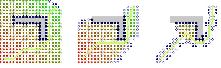
1.1 Paths generated by Dijkstra’s algorithm (left), A* search (middle), and A* search (right). . . 6
1.2 Conflict Detection and Resolution Flowchart. . . 8
1.3 Four main methods for trajectory propagation. . . 8
2.1 MM Trajectory Prediction in a “sense-and-avoid” Scenario. H1,H2, andH3denote possible hypotheses on the intruder’s predicted trajectories. . . 11
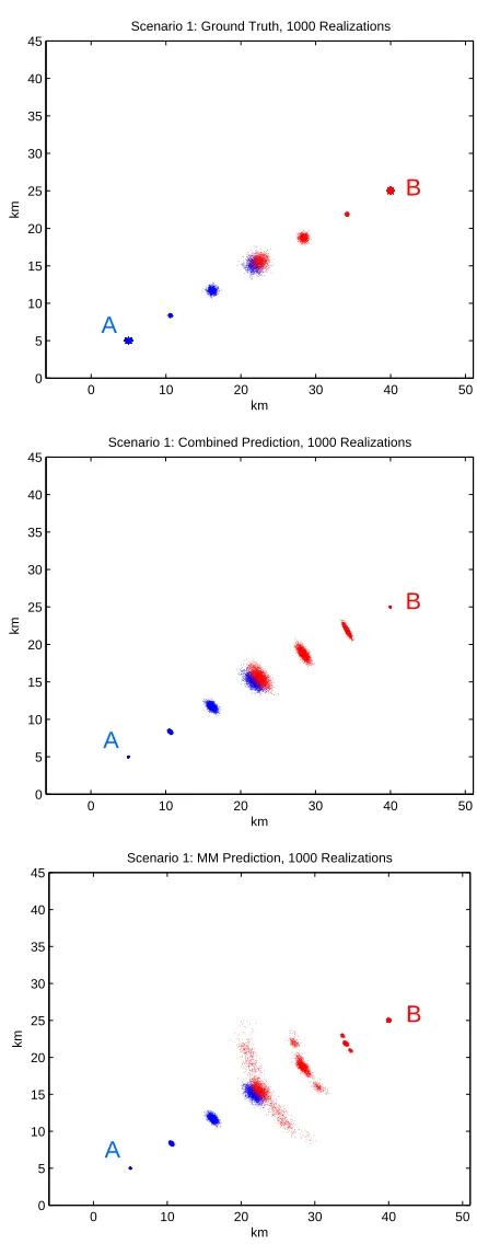
3.1 Scenario 1: Truth (top), Combined Prediction (middle) and MM Prediction (bottom) . . . . 17
3.2 Scenario 2: Truth (top), Combined Prediction (middle) and MM Prediction (bottom) . . . . 18
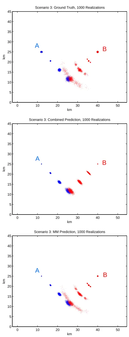
3.3 Scenario 3: Truth (top), Combined Prediction (middle) and MM Prediction (bottom) . . . . 19
3.4 Scenario 4: Truth (top), Combined Prediction (middle) and MM Prediction (bottom) . . . . 20
3.5 PC Comparison over four scenarios. MM prediction denotes the proposed (GM-based) PC prediction method, Combined Prediction denotes an existing (Gaussian-based) PC prediction method. . . 21
4.1 Model Switching Trellis withM = 5 andN = 6. . . 24
4.2 CSLVA Efficiencies. PC computations for the overlapping part of the child and parent path can be waived (top). The next best pathp(l+1) can be completely skipped over without any PC computations (bottom). . . 26
4.3 Unconstrained SLVA-based rerouting illustration. . . 28
4.4 Horizontal Scenario (H1): One Intruder (top), Two Intruders (bottom). . . 31
4.5 Horizontal Scenario (H2): One Intruder (top), Two Intruders (bottom) . . . 32
4.6 Vertical Scenario (V): One Intruder (top), Two Intruders (bottom). . . 33
5.1 Horizontal Scenario 1: One Intruder (H1 1) (top), Two Intruders (H1 2) (bottom). . . 40
5.2 Horizontal Scenario 2: One Intruder (H2 1) (top), Two Intruders (H2 2) (bottom). . . 41
5.3 Vertical Scenario: One Intruder (V1 1) (top), Two Intruders (V1 2) (bottom). . . 42
5.4 Weather Scenario: No Intruders (W1 0) (top), One Intruder (W1 1) (bottom). . . 43
Abstract
The problem of aircraft conflict detection and resolution (CDR) in uncertainty is addressed in this thesis. The
main goal in CDR is to provide safety for the aircraft while minimizing their fuel consumption and flight
delays. In reality, a high degree of uncertainty can exist in certain aircraft-aircraft encounters especially
in cases where aircraft do not have the capabilities to communicate with each other. Through the use
of a probabilistic approach and a multiple model (MM) trajectory information processing framework, this
uncertainty can be effectively handled. For conflict detection, a randomized Monte Carlo (MC) algorithm is
used to accurately detect conflicts, and, if a conflict is detected, a conflict resolution algorithm is run that
utilizes a sequential list Viterbi algorithm. This thesis presents the MM CDR method and a comprehensive
MC simulation and performance evaluation study that demonstrates its capabilities and efficiency.
Keywords: conflict detection and resolution, collision avoidance, probability of conflict, Viterbi algorithm,
Chapter 1
Introduction
1.1
Aircraft Conflict Detection and Resolution (CDR) Problem
As time progresses, global airspace is expected to become more densely packed. To address this issue, in
2012, the United States government began the implementation of a new National Airspace System called
the Next Generation Air Transportation System (NextGen) [1]. The objectives of NextGen include reducing
fuel consumption, reducing time delays for departures and arrivals, and increasing the density of the airspace
without compromising essential safety standards. Aircraft conflict detection and resolution (CDR) is one of
the underlying fields of research that will help further the development of a system such as NextGen.
The problem considered in this thesis is the unmanned aerial vehicle (UAV) sense-and-avoid (SA)
problem. In an SA scenario, a UAV, referred to as the own-ship and denoted byA, is flying around in some airspace that may also contain civilian (private or commercial) or military aircraft, referred to as intruders
and denoted by B(b), b = 1,2, . . . . While the own-ship is strictly considered to be a UAV, intruders can
be human operated aircraft or other UAVs. Within this scenario, the own-ship and the intruders are not
capable of communicating with each other, and, therefore, no flight intent information can be shared between
them.
Because of this lack of communication and the knowledge that some intruders may have human lives
onboard, the own-ship has a major responsibility to ensure that it does not collide with any of the intruders
or even come close to colliding for that matter. It realizes this collision avoidance (CA) responsibility by
using its onboard sensors to detect the current state of intruders that are in its nearby region, propagating
their trajectories into the future, evaluating the probability of a conflict occurring within the foreseen future,
and executing any maneuvers that may be necessary to maintain strict safety requirements all while trying
to get to its next waypoint. The Federal Aviation Administration (FAA) sets the minimum safety separation
requirements that all aircraft must adhere to which are currently five miles of horizontal separation and 2,000
Real-world sensors are prone to measurement error, therefore the current states of the intruders that
the own-ship receives are only estimates of their true state. Because the intruders’ flight intents are unknown
to the own-ship, their future states (i.e., possible future trajectories) are probabilistically distributed based
on the current state estimates. Using these probability distributions, a probability of conflict (PC) can be
evaluated and used to determine if an avoidance maneuver is necessary. If the PC exceeds some specified
safety threshold, then the own-ship must compute an avoidance maneuver that resolves the predicted conflict.
An avoidance maneuver can consist of maneuvering strictly in the horizontal plane, strictly in the
vertical plane, a combination of both horizontal and vertical motion, or even changing the aircraft’s speed.
In this work, only strictly horizontal and strictly vertical maneuvers were considered.
A major challenge of air traffic management (ATM) is to achieve autonomous CDR on each individual
aircraft at short and mid-ranges without the intervention of air traffic controllers. As defined in the 2011
NextGen Avionics Roadmap [29], “In self-separation airspace, capable aircraft, equipped with Automatic
Dependent Surveillance-Broadcast (ADS-B) and onboard conflict detection and alerting, are responsible for
separating themselves from one another”.
1.2
Model Predictive Control (MPC)
Model predictive control (MPC) is one method that is used to solve the CDR problem. In MPC, a dynamic
model is used to predict the future events of a system in order to optimize a control action. At every time step
k, an optimal control strategy (i.e., sequence of control actions) is computed for the duration of a finite time horizon,ktok+N. Upon acquiring a control strategy, only the first action within the strategy is executed. The time horizon is then shifted forward one time step, and the process starts all over again. Because the
time horizon is iteratively shifted forward in time, this method is also referred to as receding horizon control.
While MPC does not generally produce optimal solutions, it is very useful for online applications in which
a fast response is required.
CDR is typically performed at three different scales of the look-ahead time horizon [30]. The first
scale is long range where CDR is carried out over the time horizon of several hours across the entire national
airspace. This scale is used for the coordination of daily flight plans and schedules to ensure that no conflicts
exist at airports or en route sectors. The second scale is mid-range where CDR is carried out over the time
horizon of tens of minutes across smaller, more localized regions. This scale is used to update flight plans
mid-flight via communication with an air traffic controller (ATC) to maintain the required safety separations.
The third scale is short range where CDR is carried out over the time horizon of seconds to minutes. This
scale is used to mitigate unforeseen, near-future conflicts via an onboard collision avoidance system (CAS)
1.3
Overview of Existing Methods in the Literature
In the literature, many different approaches exist that attempt to solve the CDR problem. The most
common categories of CDR methods are geometric, force field, airspace discretization, mixed-integer linear
programming (MILP), and probabilistic [6, 12, 19].
Among all of the categories of CDR methods listed, geometric methods are the simplest and most
straightforward theoretically. Using linear projections, the future trajectories of any aircraft in the encounter
are predicted. One geometric method is called the point of closest approach (PCA) method [28], and it
consists of comparing the velocity vectors of the two aircraft to find the PCA which is then used to find
the miss distance vector between them. If the length of the miss distance vector falls below the minimum
separation distance, then the two aircraft will be turned away from each other in order to increase the space
between them.
In the PCA method, some coordination is required because one aircraft will be turned in one direction
and the other in the opposite direction. Furthermore, this method is only optimal for encounters involving
only two aircraft. As the number of aircraft in an encounter increases beyond two, the method becomes
gradually worse because the act of two aircraft fixing a predicted conflict between each other may introduce
a new conflict between a different pair of aircraft.
One geometric method that does not require any coordination is called the collision cone method [25].
In this method, a circle is placed around the obstacle or aircraft that is to be avoided. The collision cone is
formed by two lines that go from the tangents of the circle to the aircraft that is doing the avoiding. If the
velocity vector of the aircraft that is doing the avoiding is between the two tangential lines, then a future
conflict has been detected, and a resolution needs to be made. In this method, a combination of velocity,
heading, and altitude changes can be used to mitigate the conflict. However, the simplest resolution is to
make the velocity vector of the aircraft doing the avoiding match one of the two tangential lines.
The collision cone method is typically used to avoid static objects but can be extended for avoidance
of dynamic objects. Despite this method not requiring any coordination, it still suffers as the number of
aircraft in an encounter increases beyond two in the same way that the PCA method does. One way in
which the PCA method and collision cone method differ is that the PCA method produces only one option
to resolve the conflict (i.e., turn in a particle direction), whereas the collision cone method produces multiple
options, some better than others, to resolve the conflict.
Another popular geometric method which is quite similar to PCA is the reactive inverse proportional
navigation method (RIPNA) [10,13]. RIPNA is derived from the Proportional Navigation (PN) guidance law
to a missile in order to make the Line of Sight (LOS) rate of rotation between the missile and the target
zero. Making the LOS rate of rotation zero effectively means that the missile is heading directly towards its
target, and a collision is imminent.
RIPNA is essentially an inverse PN guidance law meaning that lateral accelerations are applied that
will increase the LOS rate of rotation between two aircraft thus pulling them out of a collision course. For
each pair of aircraft in an encounter, a Zero Effort Miss (ZEM) distance, the minimum distance that two
aircraft will reach if they both remain on their current trajectories, is computed along with a time-to-go, the
time until the ZEM is reached. The currently selected aircraft will only consider other aircraft with which
it has a ZEM less than some specified desired distance as potential threats. From these potential threats,
the aircraft that it has the smallest time-to-go with is avoided first followed by the aircraft with the second
smallest time-to-go and so on.
Just like with PCA, RIPNA poses the issue of resolving one conflict between a pair of aircraft only
to create a new conflict. Furthermore, while RIPNA can maintain the minimum separation distance between
aircraft, it cannot guide an aircraft to its next waypoint, and, in [10, 13], a separate guidance method called
Dubins path is used to guide an aircraft to its destination when no conflicts exist. Dubins path states that
an aircraft must turn at its maximum turn rate until its heading faces its destination. A special case exists
where an aircraft’s destination lies within the circle defined by the aircraft’s maximum turn rate. To resolve
this case, the aircraft must turn in the opposite direction until the destination lies on the edge or outside of
the maximum turn radius circle.
The most novel of the CDR methods fall arguably into the force field category. This CDR category
is derived from particle physics where repulsive and attractive forces dictate the interaction between charged
particles. Aircraft, obstacles, and aircraft destinations all act as charged particles. Aircraft and obstacles
are assigned repulsive charges, and the aircraft destinations are assigned positive charges. When an aircraft
feels the charge of another aircraft, an obstacle, or its destination, a force vector is computed using the force
vector function.
A force field method’s performance is solely dependent on the force vector function that it uses. This
function must be continuous and differentiable, must produce larger force vectors as the distance between
an aircraft and an obstacle decreases, and must produce smaller force vectors as the distance between an
aircraft and its destination decreases. Generally speaking, a force vector function is difficult to design and
implement [34, 37]. However, after obtaining a sufficient force vector function, force field methods benefit
from fast calculations. Such methods can reliably produce safe paths for aircraft to fly when the number of
aircraft is relatively small, although the safe paths are often not optimal. Because force field methods are
A few special cases exist within the force field methods. One special case occurs when an aircraft
gets stuck in a local minimum which is where the net force is either zero or very close to zero. At the expense
of computation time, when an aircraft is found to be stuck in a local minimum, some additional algorithm
is run to help the aircraft escape the local minimum. Another special case arises when generated waypoints
are unreachable or extremely difficult to reach based on the aircraft’s performance specifications, specifically
maximum turning radius.
Another category of CDR methods revolves around airspace discretization. By dividing the airspace
into discrete, uniformly spaced nodes, the CDR problem becomes one of finding an optimal path through
a weighted graph. Popular computer science search algorithms such as Dijkstra’s algorithm and A* search
can be used to efficiently find the shortest route between two points in a graph.
Dijkstra’s algorithm finds the shortest path from a given source node to every other node in a
graph [8]. When only a single shortest path is being sought, i.e., a single destination node is specified, the
algorithm stops searching when the shortest path from the source node to the destination has been found.
Dijkstra’s algorithm does not directly search in the direction of the destination node but instead gradually
explores, in a circular wavefront-like fashion, farther and farther away neighboring nodes and computing the
shortest path to each consecutive neighboring node.
A* search, an extension of Dijkstra’s algorithm, uses heuristics to make the search more efficient.
Within the CDR framework, one heuristic would be a constraint on the flying direction [35]. This constraint
would limit the searched neighboring nodes to only those that fall within a±90°radius of the direction of
the current velocity vector thus reducing the total number of nodes searched by one-third. The performance
of A* search is entirely dependent on the heuristics that are used. While Dijkstra’s algorithm guarantees
that the solution is strictly optimal, A* search does not always guarantee the same optimality but benefits
from a reduction in computational complexity.
A derivation of A* search called A* works by only exploring neighboring nodes that are within a
fixed, positivevalue of the lowest-cost neighboring node [7]. By searching fewer nodes than A*, A*further
reduces the computational complexity at the expense of optimality. Fig. 1.1 shows a comparison of the
paths generated by Dijkstra’s algorithm, A*, and A*.
In [23], the CDR problem is formulated as a classic stochastic optimal control problem where an
optimal control input is computed by approximating the stochastic differential equation of motion by a
Markov chain. The method involves time and state-space discretization which makes the computational
complexity quite high. The major caveat with methods that discretize the state-space is the tradeoff
be-tween the resolution of the discretized grid, i.e., the amount of nodes per unit length of the grid, and the
Figure 1.1: Paths generated by Dijkstra’s algorithm (left), A*search (middle), and A*search (right).
As the number of nodes per unit length increases, the computational burden of finding an optimal solution
increases exponentially. On the other hand, if the state-space is divided up into fewer but larger nodes, then
the optimality and safety of the generated path will be compromised.
The next category of CDR methods utilize the powerful optimization technique that is MILP [7, 12,
32]. MILP models obstacles, collision avoidance rules, and no-fly zones as logical (integer) constraints and
an aircraft’s performance limitations as continuous constraints. Open-source and commercial optimization
software packages are available that can solve the full set of equations and produce minimum flight-time,
collision-free trajectories for all aircraft involved in the scenario. In the MILP framework, the trajectories
of all aircraft in an encounter are optimized jointly, in other words for the “greater good.”A trajectory
optimized in this way may be suboptimal for an individual aircraft, but the sum of the trajectories of all
aircraft is globally optimal.
The attractive feature of MILP is that it is guaranteed to find the most optimal feasible solution
granted that at least one feasible solution exists. The significant drawback of MILP methods is that they are
practically infeasible for real-time CA because the computation time is too high. On top of that, the time
complexity to solve a set of MILP equations increases as more constraints are added. This increase in time
complexity contrasts with a method such as A*search which would benefit from an increase in constraints.
The last CDR category that will be discussed consists of the probabilistic methods. Probabilistic
methods use the uncertainties inherent in the dynamic model to predict the possible future trajectories of
aircraft over a finite time horizon. Each possible future trajectory is weighted depending on its probability
of occurring. Probabilistic approaches are reasonable because they provide a good tradeoff between relying
too heavily on an aircraft sticking to its original flight plan vs. relying too heavily on an aircraft performing
worst-case maneuvers. Within a probabilistic approach, decisions for CR are made based on the fundamental
likelihood of a conflict, i.e., the PC.
deci-sion process (POMDP) [3, 38]. In a Markov decideci-sion process (MDP), the state of the system (i.e., positions
and velocities of all aircraft) changes probabilistically based on the current states and actions of the aircraft
involved. In a POMDP, the state of the system is now expressed in terms of observations (i.e., an estimation
of an aircraft’s state) which are probabilistically generated and conditioned on the current states and
ac-tions of the aircraft involved. The observaac-tions all together form a belief, a probability distribution over all
possible system states. Solving a POMDP consists of computing a policy that selects actions in a way that
either maximizes an expected reward or minimizes an expected cost. The policy accounts for the current
uncertainty in the system (i.e., exact positions and velocities of intruder aircraft are not exactly known) and
the future uncertainty about how the system will evolve (i.e., what maneuvers might the intruders make).
POMDP algorithms generally require discretization of the state-space in order to be able to compute
an optimal control policy. State-space discretization imposes a computational burden that can render these
types of algorithms useless for practical implementation. By using Monte Carlo (MC) methods, the
compu-tational problems introduced by discretizing the state-space can be relieved. In [3], a MC Value Iteration
algorithm was used to solve the POMDP in the continuous state-space.
MC methods account for probabilistic uncertainty due to disturbances, uncertain state estimation,
modeling error, and stochastic mode transitions. As a result, they are well suited for solving
chance-constrained (i.e., the probability of failure must be below a certain threshold) stochastic optimal control
problems. A finite number of particles are used to approximate all aircraft states as probability
distribu-tions. Through this approximation, an intractable stochastic optimization problem can be transformed into
a tractable deterministic optimization problem. By solving the deterministic problem, a solution that
ap-proximates the original stochastic problem can be found. The approximation error decreases as the number
of particles increases. Also, particle-based methods such as MC are able to handle arbitrary probability
distributions.
[4,9,18] proposed solutions to the stochastic MPC problem by using sequential Monte Carlo (SMC).
SMC is similar to simulated annealing in that it is capable of producing a globally optimum solution given
a non-convex optimization problem that may have several local minima or maxima. SMC extends MC by
adding a resampling process wherein the particles of a probability distribution are continually resampled
to allow them to converge to the global optimizer. Despite MC methods fixing the problem of having to
discretize the state-space, their computational complexity can still be very high. The body of work within
this thesis follows a probabilistic approach based around MC which provides a general and systematic way
to handle the uncertainties that exist within the CDR problem.
Fig. 1.2 shows the process of CDR for a probabilistic method. The first step for the own-ship is to
a dynamic model, the own-ship can find the predicted states of the detected aircraft. For conflict detection,
the predicted states are used to obtain a PC between the own-ship and every other aircraft. If any one of
the calculated PCs exceeds a specified safety threshold, then conflict resolution is required. Otherwise, the
own-ship and all other aircraft progress one time step into the future along their original flight paths.
State Estimation Environment
Current States
PC ≥ δ ?
Dynamic Model Predicted States Conflict Detection PC Yes Conflict Resolution
No
Figure 1.2: Conflict Detection and Resolution Flowchart.
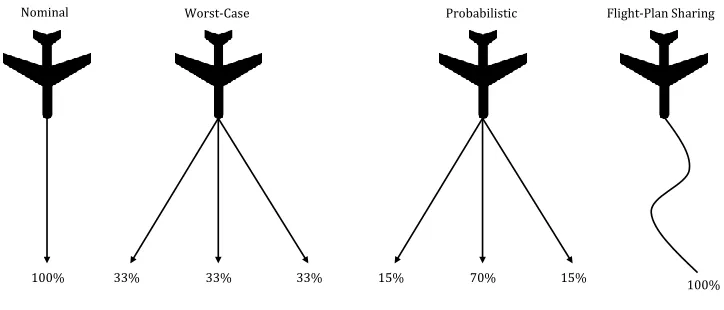
Across all of the categories of CDR methods, many ways exist for projecting an intruder’s current
information into the future. The four main methods of trajectory propagation are nominal, worst-case,
probabilistic, and flight-plan sharing. The nominal method projects current states into the future without
the consideration of disturbances or flight-plan changes. An intruder’s position is simply extrapolated based
on it’s current velocity vector or rate of turn. The worst-case method assumes that an intruder will perform
any range of maneuvers with equal probability. This method is extremely conservative because in some cases
a conflict may be declared for a projected trajectory that is very unlikely to happen in a real-world situation.
The probabilistic method constructs a set of possible future trajectories where each trajectory is assigned
a probability of occurring. In the flight-plan sharing method, all aircraft share their flight intents with one
another. This sharing of information makes the CA problem mush easier. As technology progresses and
becomes more widely available, the flight-plan sharing method will see more and more attention. Fig. 1.3
illustrates the four main trajectory propagation methods.
Nominal Worst-Case Probabilistic Flight-Plan Sharing
100% 33% 33% 33% 15% 70% 15% 100%
Chapter 2
Multiple Model (MM) CDR
Framework
The MM framework and algorithms for CDR presented in this thesis were originally proposed and developed
in our papers [15–17].
2.1
Aircraft Model
The characteristic motion models of an aircraft can be classified into the following kinematic categories [20].
In the horizontal plane, the categories are constant velocity (CV) (i.e., straight line motion), constant
acceleration (CA) (i.e., speed up/slow down), and constant turn (CT) (i.e., left/right). In the vertical plane,
the categories are constant height (CH) (i.e., level cruise) and constant climb/descent (CD). A flight mode
is then modeled as a combination of a horizontal and a vertical model. Flight dynamics are described by
a hybrid system (HS) model which includes a set of flight models and the rules that govern the transition
between these flight models.
Consider the Markov Jump Linear System (MJLS) shown below:
xk =Fmkxk−1+Gmkwk (2.1)
zk =Hmkxk+vk (2.2)
wherek= 1,2, . . .is the time index,xk ∈Rnxis the continuous kinematic state,mk∈M=m(1), m(2), . . . , m(M) is the discrete modal state, zk ∈ Rnz is the sensor measurement, and w
k ∼ N(0, Qk) and vk ∼ N(0, Rk)
are mutually independent white process and measurement noises, respectively. For the own-ship, the model
assumed to be a Markov chain with the following transition and initial probabilities:
P{mk =m(j)|mk−1=m(i)}=πij (2.3)
P{m0=m(i)}=µ (i)
0 (2.4)
A CA kinematic model is not used in this work. However, CV (2.5) and CT (2.6) kinematic models
are used and are shown below [20]:
xk =
1 T 0 0
0 1 0 0
0 0 1 T
0 0 0 1
xk−1+ T2 2 0 T 0 0 T22
0 T
wk (2.5)
xk =
1 sinωωT 0 −1−cosωωT 0 cosωT 0 −sinωT
0 1−cosωT ω 1
sinωT ω
0 sinωT 0 cosωT
xk−1+Gwk (2.6)
where xk = [ x ˙x y ˙y ]0 is the state vector,T is the time step duration,ω is a constant turn rate (i.e.,
control input), andwk is the process noise. Note that CV = lim ω→0CT(ω).
The CH/CD model that is used is shown below:
xk=
1 T 0
0 1 0
0 0 1
xk−1+ 0 0 T
vk+
T2 2 0 T 0 0 T22
wk (2.7)
wherexk= [ x ˙x z ]0 is the state vector,T is the time step duration,vk ∈v(1), . . . , v(5) are the constant
climb/descent rates (i.e., control inputs), andwk is the process noise.
2.2
Multiple Model (MM) Trajectory Prediction
Multiple model (MM) trajectory prediction is the new and innovative way to handle the many challenges
that exist in aircraft trajectory prediction. It is widely accepted because of its ability to effectively handle
multiple modes of operation [21]. It is also capable of providing good approximations of highly nonlinear
as aircraft intent and various flight modes. Fig. 2.1 illustrates an SA scenario where the own-ship needs to
predict the trajectory of an intruder under uncertainty of the intruder’s intent (for possible maneuvers) in
order to avoid a conflict.
Figure 2.1: MM Trajectory Prediction in a “sense-and-avoid” Scenario. H1, H2, and H3 denote possible
hypotheses on the intruder’s predicted trajectories.
In a probabilistic trajectory prediction, the main goal is to approximate as accurately as possible
the PDFsf(xk+n|zk),n = 1, . . . , N, where k is the current time, zk ={z1, . . . , zk} is the available sensor
data, and N is the look-ahead time horizon for how far into the future predictions are made. MM filters such as GPB, IMM, or VSMM [21] provide state estimates ˆx(ik)
k|k, associated covariances P
(ik)
k|k and model
probabilitiesµ(ik)
k|k,ik = 1, . . . M whereM is the number of discrete modal states. The MM filter density is
approximated as a Gaussian mixture (GM):
f(xk|zk) = M
X
ik=1
µ(ik)
k|kN
xk; ˆx
(ik)
k|k, P
(ik)
k|k
(2.8)
Furthermore, the prediction is based on the motion model given by (2.1) and (2.3) with ˆx(ik)
k|k,P
(ik)
k|k ,
andµ(ik)
k|k being the “initial” condition.
Let a model sequence in the time interval [k, k+N] be denoted by
Mkk+N ,(m(ik)
k , . . . , m
(ik+N)
k+N )∈M
N+1 (2.9)
whereik:k+N ,(ik, . . . , ik+N) is the underlying sequence of model indices.
Then
f(xk+N|zk) =
X
ik:k+N
where
f(xk+N|Mkk+N, z k) =
Nxk+N; ˆx
(ik:k+N)
k+N|k , P
(ik:k+N)
k+N|k
(2.11)
P{Mkk+N|zk}=µ(ik)
k|kπikik+1. . . πik+N−1ik+N (2.12) and ˆx(ik:k+N)
k+N|k , P
(ik:k+N)
k+N|k are obtained recursively by the Kalman filter prediction equations for each model
sequenceMkk+N with the initial ˆx(ik)
k|k, P
(ik)
k|k .
2.3
Weather Model
Along with aircraft-aircraft encounters, aircraft-weather encounters are also taken into account in which the
own-ship is given data of bad weather cells that lie along its intended flight path. As in the aircraft-aircraft
encounters, the own-ship must perform any necessary maneuvers to avoid conflicts with the bad weather.
Based on four-dimensional predicted weather data (available from a weather service repository, such as the
METOC Data Server (MDS)), the spatial density and concentration (severity) of the bad weather can be
obtained. Modeling the bad weather concentration as a spatial random variableξ, the spatial density can be viewed as a probability density, and the PDFs ofξ can be constructed by GM fitting of the spatial density data:
fξ(pk+n) = Lk+n
X
l=1
µ(kl+)nN(pk+n; ¯p
(l)
k+n, C
(l)
k+n) (2.13)
Chapter 3
Conflict Detection (CD)
The MM-based approach and algorithm for CD presented in this chapter were proposed in our paper [16].
3.1
Predicted Probability of Conflict (PC)
Most probabilistic methods for estimating the probability of conflict (PC) in the literature assume that the
predicted separation vector between two aircraft is a Gaussian distribution. In an advanced multiple model
trajectory prediction framework, however, the separation vector has a Gaussian mixture distribution, and
approximating it by a single Gaussian, as in [14, 22, 40], leads to significant inaccuracies of the predicted
PC in a highly uncertain environment. This chapter presents a more accurate method, proposed in [16], for
estimating PC by utilizing the information from multiple model aircraft trajectory prediction.
PC is the probability that the distance between two aircraft falls below a specified minimum
sepa-ration distance. As specified by the current aviation standards, the horizontal (2D) and vertical sepasepa-ration
distances (1D) are commonly treated separately, [27,30], which amounts to a cylindrical protected zone. A 3D
ellipsoidal protected zone, proposed in [5,22], where the horizontal and vertical separations are treated jointly
is considered here. More specifically, letAandBdenote two aircraft with position vectorsxA= (xA,yA,zA)0
and xB = (xB,yB,zB)0 in an inertial (East-North-Up) Cartesian coordinate system Oxyz, and let the
dis-tance vector be ρAB =xA−xB. If λxy and λz are the given horizontal and vertical separation thresholds, respectively, the “weighted” distance vector is ΛρAB, where Λ = diag{1/λxy,1/λxy,1/λz}, and the ellipsoidal protected zone is defined as
Rλ=
ρ∈R3:kΛρk ≤1 (3.1)
wherekak= (a0a)12 is the Euclidean norm of a vectora.
If fρABk(ρ) is the probability density function (PDF) of the distance vector ρABk at time k, then the instantaneous PC is
P Ck=P{kΛρABkk ≤1}=
Z
Rλ
and the maximal PC over a time interval (k, k+N] is
P C(k,k+N]= max
0<n≤NP Ck+n (3.3)
In the CDR problem,kis the current time andNis the length of the time horizon. The corresponding predicted PC is computed via (3.2) and (3.3), respectively, based on predicted densities ˆfρABk
+n(ρ|z
k)
≈
fρABk
+n(ρ),n= 1,2, . . . , N, wherez
k =
{z1, . . . , zk}is the available sensor data.
Let
xA∼fxA(x) =
MA
X
i=1
µA(i)Nx; ˆxA(i), PA(i) (3.4)
xB∼fxB(x) =
MB
X
j=1
µB(j)Nx; ˆxB(j), PB(j) (3.5)
IfxA andxB are independent, thenρAB also has a GM distribution, given by
ρAB∼fρAB(ρ) =
MAB
X
l=1
µAB(l) Nρ; ˆρAB(l), PAB(l) (3.6)
where MAB = MAMB, µ
(l)
AB = µ
(i)
Aµ
(j)
B , ˆρ
(l)
AB = ˆx
(i)
A −xˆ
(j)
B , P
(l)
AB = P
(i)
A +P
(j)
B and the single index l =
1, . . . , MAB is correspondent to the double index (i, j),i= 1, . . . , MA,j= 1, . . . , MB.
3.2
Computing the Predicted PC
The randomized algorithm, given in Algorithm 1, is used to estimate the instantaneousP Ck. This algorithm
is based on the direct estimation of PC by the definition (3.2) with (3.6).
Algorithm 1Randomized Algorithm for EstimatingP Ck+n
1: ChooseNM C, number of MC runs
2: SetP Cdk+n = 0
3: forr= 1 to NM C do
4: Sample random index l∼nµ(ABl)
k+n:l= 1, . . . , MABk+n
o
5: Sample random vectorρ∼ Nρ; ˆρ(ABl)
k+n, P
(l)
ABk+n
6: if kΛρk ≤1then
7: P Cdk+n =dP Ck+n+ 1
8: P Cdk+n=P Cdk+n/NM C
The good approximation properties (in a probabilistic sense) of the randomized estimation of PC
are discussed in [30, 31, 39], wherein quantitative bounds on the approximation error can be found. In the
3.3
PC Estimation Accuracy Evaluation
The performance of the proposed GM-based PC prediction method is compared, through simulation, with
a traditional Gaussian-based approach over an SA UAV encounter scenario. The results demonstrate and
quantify the improvement achieved by the proposed CD method.
Several SA encounter scenarios, as illustrated in Fig. 2.1, were simulated where the own-ship predicts
the trajectory of an intruder under uncertainty of the intruder’s intent in order to avoid a conflict. More
and more research has been focused on SA recently since SA capability is required for UAVs to be able to
operate in civil airspace [38].
For simplicity, the scenarios are contained within the horizontal plane Oxy. The own-ship, A, is assumed to have a constant velocity (CV) motion, while the intruder,B, can have either a CV or a constant turn (CT) motion. An intruder B is modeled through the hybrid system (2.1), (2.3), (2.4) and has three motion models which are m(1) = CV (straight) withω(1) = 0o/s, m(2)= CT (left turn) with ω(2)= 1o/s,
and m(3) = CT (right turn) with ω(3) =
−1o/s. The flight mode initial and transition probabilities are
µ(1)0 = 0.8, µ(2)0 = 0.1, µ(3)0 = 0.1 and π11 = 0.8, π12 = 0.1, π13 = 0.1, π21 = 0.9, π22 = 0.1, π23 =
0.0, π31= 0.9, π32= 0.0, π33= 0.1. The time step duration isT = 20 sec, and the process noise covariance
isQ=q2Iwithq= 5m/s2.
Four scenarios are presented each with different aircraft geometries that are generated according
to the aforementioned models. In each scenario, the amount of Monte Carlo runs (i.e., the number of
random trajectories generated) isNM C = 1000, and the time horizon is 60 sec. PC is estimated as the ratio NC/NM C, the number of runs where a conflict occurredNC over the total number of runs performedNM C.
The minimum horizontal separation distance that defines a conflict isλxy = 1km.
The predicted PC is computed using the proposed algorithm, Algorithm 1, which is based on MM
trajectory prediction (2.10)–(2.12) and is referred to as MM prediction in all of the results. For the purpose
of comparison, the predicted PC is also computed through the algorithm of [14, 22, 40] where MM trajectory
prediction is still used but the predicted GM is approximated by a single Gaussian matching the mean and
covariance of the mixture. PC predicted in this way is referred to as combined prediction in all of the
results. With this Gaussian approximation, integral (3.2) is computed in the simulation by the randomized
PC estimation algorithm of [30].
Fig. 3.1 shows the scatter plots for the ground truth (top), the combined prediction (middle), and
the MM prediction (bottom) in Scenario 1. In this scenario, the intruder follows a nearly CV motion which
means that it does not take any turns and is only acted upon by a random process noise. The combined
accounts for possible maneuvers made by the intruder. For this scenario, the true PC is 0.2, combined
prediction PC is 0.24, and MM prediction PC is 0.15. In this particular case, the combined prediction
achieved a slightly more accurate predicted PC than the MM prediction did because the intruder’s true
position density is already Gaussian.
Fig. 3.2 shows the results for Scenario 2. In this scenario, the intruder follows a random sequence
of nearly CV and CT motion models that are chosen according to the transition probabilities previously
provided. In this particular case, MM prediction better approximates the true Gaussian distribution over
combined prediction because the true distribution here is in fact a GM. The combined prediction
approxi-mates the true PC fairly poorly. The true PC is 0.25, combined prediction PC is 0.365, and MM prediction
PC is 0.248. As expected, when more uncertainty is present in a scenario, combined prediction fails as
opposed to MM prediction which very accurately predicts PC.
Scenarios 3 and 4 are shown in Figs. 3.3 and 3.4, respectively. As observed in Scenario 2 and all
other scenarios that involve random maneuvers for the intruder, MM prediction more accurately estimates
the true PC than combined prediction does.
Finally, Fig. 3.5 compares, over all four scenarios, the predicted PC as computed by the proposed
method (MM Prediction) and an existing method (Combined Prediction) against the true PC. For the case
in which the intruder makes no maneuvers, both PC prediction methods are comparable. However, for the
cases that involve more serious uncertainty about the intruder’s motion intent, the proposed PC prediction
0 10 20 30 40 50 0
5 10 15 20 25 30 35 40 45
km
km
Scenario 1: Ground Truth, 1000 Realizations
A
B
0 10 20 30 40 50
0 5 10 15 20 25 30 35 40 45
km
km
Scenario 1: Combined Prediction, 1000 Realizations
B
A
0 10 20 30 40 50
0 5 10 15 20 25 30 35 40 45
km
km
Scenario 1: MM Prediction, 1000 Realizations
A
B
10 20 30 40 50 0
5 10 15 20 25 30 35 40 45
km
km
Scenario 2: Ground Truth, 1000 Realizations
A
B
10 20 30 40 50
0 5 10 15 20 25 30 35 40 45
km
km
Scenario 2: Combined Prediction, 1000 Realizations
A
B
10 20 30 40 50
0 5 10 15 20 25 30 35 40 45
km
km
Scenario 2: MM Prediction, 1000 Realizations
A
B
0 10 20 30 40 50 0
5 10 15 20 25 30 35 40 45
km
km
Scenario 3: Ground Truth, 1000 Realizations
A
B
0 10 20 30 40 50
0 5 10 15 20 25 30 35 40 45
km
km
Scenario 3: Combined Prediction, 1000 Realizations
A
B
0 10 20 30 40 50
0 5 10 15 20 25 30 35 40 45
km
km
Scenario 3: MM Prediction, 1000 Realizations
A
B
10 20 30 40 50 60 0
5 10 15 20 25 30 35 40 45
km
km
Scenario 4: Ground Truth, 1000 Realizations
A
B
10 20 30 40 50 60
0 5 10 15 20 25 30 35 40 45
km
km
Scenario 4: Combined Prediction, 1000 Realizations
A
B
10 20 30 40 50 60
0 5 10 15 20 25 30 35 40 45
km
km
Scenario 4: MM Prediction, 1000 Realizations
A
B
1 2 3 4 0
0.05 0.1 0.15 0.2 0.25 0.3 0.35 0.4
PC comparison for different scenarios
Scenarios
Probability of Conflict
PC: Ground Truth PC: MM Prediction PC: Combined Prediction
Chapter 4
Conflict Resolution (CR)
The MM formulation for CR and the optimal constrained sequential list Viterbi algorithm presented in this
chapter were proposed in our paper [17].
4.1
When is CR Needed?
It is assumed that, at each time k (current time), all filtered estimates ˆxAk|k and ˆxBb
k|k, b = 1,2, . . ., are
available. The CD strategy, detailed in Section 3.1, is used to predict the GM PDFs of all intruders and,
given the own-ship mode sequenceMkk+N, compute the predictedP Ck(b+)n,n= 1, . . . , N; b= 1,2, . . . ,where
N is the look-ahead time horizon andb denotes intruderBb.
A conflict alert is triggered “ON” iff
max
(b,1≤n≤N)P C (b)
k+n≥δ (4.1)
whereδis a threshold.
Upon a conflict alert, the current mode sequence Mkk+N of the own-ship needs to be updated to provide safety (i.e., to guarantee max(b,1≤n≤N)P C
(b)
k+n< δ along the updated flight path).
4.2
Constrained Optimization: Maneuvering Cost Function
Let ck+n(m(i), m(j)), i, j ∈ {1,2, . . . , M} be the cost of switching from mode m(i) at time k+n−1 to
modem(j)at timek+n, n= 1,2, . . . , N. Then, the collision avoidance (CA) problem is formulated as the
following “chance-constrained” stochastic MPC problem:
Minimize:
J(Mkk+N) =
N
X
n=1
subject to:
P Ck(b+)n< δ, n= 1, . . . , N; b= 1,2, . . . (4.3)
It is clear that the formulation of the total cost, given by (4.2), has some limitations. It only
takes into account the costs for switching between flight modes and does not include any information about
the own-ship’s destination. The lack of destination information in the objective function leaves the CDR
problem “half-solved” in a way because some extra guidance algorithm is required to drive the own-ship to
its destination in the absence of conflicts. Likewise, based on (4.2) alone, the own-ship is not capable of
returning to the originally intended flight plan or flight altitude. Although, careful design of the cost matrix
may allow the own-ship to partially control its trajectory. The one property that is guaranteed as a result
of (4.2) and (4.3) is that the overall trajectory of the own-ship will be conflict-free.
Despite these limitations, a strong argument still supports this formulation. First, the primary goal
in CDR is to guarantee the safety of the aircraft involved in a close encounter. Trajectory optimization
comes second meaning that only once a conflict is resolved will the own-ship be allowed to return to the
original flight path or be re-routed to the next waypoint.
More terms could be added to the objective function to remedy such limitations. The only problem
is that having more terms that need to be optimized can lead to drastic increases in the complexity of the
resulting stochastic optimal control problem which can require extensively more computational resources.
For many practical applications, e.g., UAV SA, the computational resources are quite limited. From this
viewpoint, the formulation and approach, proposed in [17], that is presented in this chapter is quite attractive.
4.3
Viterbi Algorithm (VA) & Sequential List VA (SLVA)
The unconstrained optimization problem (4.2) is one of finding a best (least costly) path through a trellis
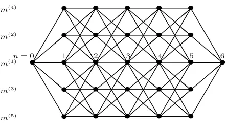
digraph. Fig. 4.1 illustrates a typical model switching trellis (at current timek) withM = 5 models (nodes) and look-ahead time horizonN = 6 (i.e., ending time isk+N). Without loss of generality, it is assumed that at the start and end times (kand k+N, respectively) the own aircraft is in flight modem(1), CV motion.
As discussed later in Section 4.5), a complete trellis withm(3), m(5)being right CT models andm(2), m(4)
being their symmetrical left CT models is used. The depicted trellis is not complete because switching from
a left CT to a right CT (and vise versa) is only possible through the CV model.
Finding an unconstrained best path through a trellis can be easily and efficiently done via Dynamic
Programming, e.g., via the popular Viterbi algorithm (VA) [11]. The constrained problem (4.2)–(4.3) is
more complicated. The obvious idea of searching for a best path, after determining the feasible
m(4)
m(2)
m(1)
m(3)
m(5)
n= 0✁✁ 1 2 3 4 5 6
✁✁ ✁✁ ✁
•
•
•
❅ ❅ ❅❅ ❆ ❆ ❆ ❆ ❆ ❆ ❆ ❅ ❅ ❅❅ ✁✁ ✁✁ ✁✁ ✁•
•
•
❅ ❅ ❅❅ ❆ ❆ ❆ ❆ ❆ ❆ ❆ ❅ ❅ ❅❅ ✁✁ ✁✁ ✁✁ ✁•
•
•
❅ ❅ ❅❅ ❆ ❆ ❆ ❆ ❆ ❆ ❆ ❅ ❅ ❅❅ ✁✁ ✁✁ ✁✁ ✁•
•
•
❅ ❅ ❅❅ ❆ ❆ ❆ ❆ ❆ ❆ ❆ ❅ ❅ ❅❅ ✁✁ ✁✁ ✁✁ ✁❆ ❆ ❆ ❆ ❆ ❆ ❆ ❅ ❅ ❅❅•
•
•
•
•
•
❅ ❅ ❅❅ ❆ ❆ ❆ ❆ ❆ ❆ ❆•
•
•
❅ ❅ ❅❅ ❆ ❆ ❆ ❆ ❆ ❆ ❆ ❅ ❅ ❅❅ ✁✁ ✁✁ ✁✁ ✁•
•
•
❅ ❅ ❅❅ ❆ ❆ ❆ ❆ ❆ ❆ ❆ ❅ ❅ ❅❅ ✁✁ ✁✁ ✁✁ ✁•
•
•
❅ ❅ ❅❅ ❆ ❆ ❆ ❆ ❆ ❆ ❆ ❅ ❅ ❅❅ ✁✁ ✁✁ ✁✁ ✁•
•
•
❅ ❅ ❅❅ ❆ ❆ ❆ ❆ ❆ ❆ ❆ ❅ ❅ ❅❅ ✁✁ ✁✁ ✁✁ ✁ ✁✁ ✁✁ ✁✁ ✁•
Figure 4.1: Model Switching Trellis withM = 5 andN = 6.
paths. Since the PC evaluation is the computational bottleneck in this problem, a better idea is to organize
the search of the best paths in a sequential manner (in an increasing order of costs) and then check feasibility
so that PC is only evaluated over lower-cost candidate paths. To put it simply, the strategy is to find the
best path and check its feasibility. If it is not feasible, then the second best path is found, and its feasibility
is checked. If the second best path is infeasible, the search continues for the third best path and so on and
so forth until a path is found which is feasible.
The problem of finding theLbest paths through directed graphs has been well studied in the area of computational geometry and many general algorithms exist. More efficient algorithms, particularly tailored
to the special case of trellis graphs are available in the communications literature, [26,33,36], where algorithms
for finding theLbest paths through a trellis are generally referred to as the List Viterbi Algorithms (LVAs). For the purpose of finding an optimal solution to the constrained problem (4.2)–(4.3), in principle, any LVA
can be used. However, the sequential LVA (SLVA) [36] best suits the problem at hand for two reasons:
1) it finds the next best path recursively based on the previous best paths, and 2) the search is organized
via forward VA-like passes through the trellis, which allows already computed PCs to be reused along the
conflict-free parts of future VA passes.
For simplicity, let the trellis states be denoted by i ∈ {1,2, . . . , M} (instead of the previous MM notationm(i)
∈M). The initial state of the trellis at timen= 0 is assumed to be 1. Letλ(ni)be the minimum
cost to reach state i at time n (from the known state 1 at time n= 0), and jn(i) ∈ {1,2, . . . , M} be the
state occupied at timen−1 by the best path into stateiat timen.
In SLVA, thelth best pathp(l)is found in a sequential manner based on the previously found (l
−1)
best pathsp(1), p(2), . . . , p(l−1)which are sorted in a non-decreasing order of costs.
where SLVA symbolizes one recursive step of the algorithm. The first step of SLVA is to obtain the best
path,p(1), via VA. VA is explained in detail in Algorithm 2. Then, usingp(1),p(2) can be found by mutating
p(1)with only one forward, cheapest cost split point. If any other split points occur when mutatingp(1) into
p(2), then p(2) cannot be the next best path because it will have a higher cost than a path that has only
one, cheapest cost split point fromp(1). Furthermore, an issue may arise where multiple paths mutate from
a previous best path with the same cost increase making all of them valid candidates to be the next best
path. This issue is solely governed by the costs assigned between the nodes in the trellis.
So, ifi∗nis the state occupied byp(1) at timen,the forward cost-to-goλ(i∗n)
n (2) ofp(2)can be written
as
λ(i
∗
n)
n (2) = min{(λ
(i∗n−1)
n−1 +cn(in∗−1, i∗n)), min
0≤j≤M, j6=i∗
n
(λ(nj−)1+cn(j, i∗n))} (4.5)
The first term in (4.5) represents the 2nd best path toi∗
n which has merged top(1)no later than timen−1.
The second term represents the 2nd best path toi∗n which has merged top(1) no earlier than timen.In the
forward pass of the algorithm, the one with the minimum cost remains in contention to becomep(2), and the
time of the last best merge,nm, is recorded. Then, p(2) is the 2nd best path to timenm−1 as determined
by the above recursion and is equal top(1) from timen
m until the end. Findingp(3) fromp(1) andp(2) can
be organized in a similar manner. A formal, more detailed description of the algorithm is given in [36].
Algorithm 2Viterbi Algorithm
Initialization:
1: fori= 1 to M do
2: λ(1i)=c1(1, i) 3: j1(i) = 1
Recursion:
4: forn= 2 to N−1 do
5: fori= 1 to M do
6: λ(ni)= min
1≤j≤M(λ
(j)
n−1+cn(j, i))
7: jn(i) = arg min
1≤j≤M
(λ(nj−)1+cn(j, i))
Termination:
8: λ(1)N = min
1≤j≤M(λ
(j)
N−1+cN(j,1))
9: jN(1) = arg min
1≤j≤M
(λ(Nj)−1+cN(j,1))
Backtracking:
10: i∗N = 1
11: forn=N−1 to 1do
12: i∗n =jn+1(i∗n+1)
Best Sequence:
13: (1, i∗
4.4
Constrained Sequential List Viterbi Algorithm (CSLVA)
For this CDR method, CD is done by the PC prediction method discussed in Chapter 3 and simply
im-plements (4.1). CR is done by the SLVA search strategy that was discussed in the previous section. A
straightforward implementation of the standard SLVA search strategy which is where PC is computed for
the entire time horizon of each next best pathp(l) would lead to many duplicate computations of the same
PC becausep(l)has portions of itself that are also present in its children (p(l+1), p(l+2), . . .). To remedy this
careless misuse of computational resources, two efficiency improvements are added to SLVA. By storing the
split times and conflict times of subsequent paths as the search runs, the same PC will never be computed
twice, and some next best paths can even be completely skipped over without computing any PCs at all
because it will be already known that they are infeasible. These two efficiency improvements are illustrated
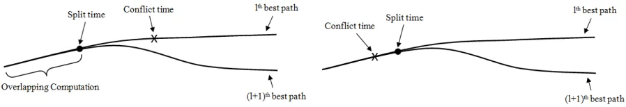
in Figure 4.2, and Algorithm 3 shows the step-by-step algorithm for the CDR method.
Figure 4.2: CSLVA Efficiencies. PC computations for the overlapping part of the child and parent path can be waived (top). The next best path p(l+1) can be completely skipped over without any PC computations (bottom).
Because the CDR method in this chapter operates off of (4.2) which lacks information about the
own-ship’s destination, an extra algorithm is executed in the absence of conflicts to reroute the own-ships’s
trajectory towards its destination. This rerouting algorithm is simple and intuitive but not efficient. It
is basically an unconstrained SLVA search where each next best path that is found is linearly projected
outwards for a fixed distance in order to “search” for the destination. The first path in the SLVA search
that is found to have a point that lies within a specified distance threshold of the destination’s position
is chosen as the rerouted trajectory, and the rerouted trajectory is terminated at the point that “hit” the
destination. The computational cost of this rerouting method depends on many factors such as the number
of discrete modal states, length of the look-ahead time horizon, turning limitations of the own-ship, and
geometry between the own-ship and destination at the time of rerouting. Fig. 4.3 illustrates this rerouting
method and shows what paths within the trellis would be considered acceptable for rerouting the own-ship
Algorithm 3Proposed CDR Algorithm At timek:
Initialization:
1: l= 1
2: p(1)= (1,1, . . . ,1)
Conflict Detection:
3: forn= 1 to N do
4: forb = 1,2,. . . do
5: ComputeP Ck(b+)n(p(l))
6: if P Ck(b+)n(p(l))≥δthen
7: Go to 10:
8: k=k+ 1
9: Go to 1:
Conflict Resolution: (Search trellis for best CR maneuver sequence)
a)Find conflict times:
10: forb = 1,2,. . . do
11: n(cb)(p(l)) = min
1≤n≤N{n:P C
(b)
k+n(p
(l))
≥δ}
b)Find next best path & split times:
12: l=l+ 1
13: p(l)= SLVA(p(1), p(2), . . . , p(l−1))
14: forj = 1 to l−1do
15: n(sl|j)= min
0≤n≤N{n:p
(l)diverges fromp(j)
}
c)Find largest split time from conflict-free parent subsequence:
16: n(l|j0)
s = min
1≤j≤l−1{n (l|j)
s :n(sl|j)< nc(b)(p(j))}
17: if n(l|j0)
s =∅ then
18: Go to 10:
19: forn=n(l|j0)
s +1 toN do
20: forb = 1,2,. . . do 21: ComputeP Ck(b+)n(p(l)) 22: if P Ck(b+)n(p(l))
≥δthen
23: Go to 10:
24: CR sequence = p(l), recalculate guidance from state at time k+N to next WP (or destination). 25: Go to 3:
4.5
Computational Efficiency Evaluation
The performance of the CR method, CSLVA, is compared, through simulation and data analysis, with a
standard implementation of SLVA over SA UAV encounter scenarios that were previously described in Section
3.3. The results clearly show the feasibility of and computational efficiency improvements achieved by the
CSLVA.
Two types of encounter scenarios are considered, one in which the own-ship makes strictly horizontal
resolution maneuvers and one in which the own-ship makes strictly vertical resolution maneuvers. The
Waypoint
Set of acceptable rerouting paths
Current position
Figure 4.3: Unconstrained SLVA-based rerouting illustration.
left turn) with ω(2) = 1o/s, m(3) = CT (soft right turn) with ω(3) =
−1o/s, m(4) = CT (hard left turn)
withω(4)= 2o/s, andm(5)= CT (hard right turn) with ω(5) =
−2o/s, where ωis the turn rate.
The model transition costs used are
c(i, j) =|ω(j)−ω(i)|, i, j= 1, . . . ,5 (4.6)
where m(1) is the initial and final trellis state as seen in Fig. 4.1. The look-ahead time horizon is N = 10 for all scenario types in this section.
Each intruder B is modeled through the same hybrid system with the same initial and transition probabilities that is described in Section 3.3. The time step duration is T = 5 sec, and the process noise covariance and number of MC runs are the same as in Section 3.3. The minimum horizontal separation
distance that defines a conflict is λxy = 5km, and the threshold on PC for triggering a conflict alert is
δ= 10−3.
Figs. 4.4 and 4.5 show two scenarios with one intruder (top) and two intruders (bottom), respectively.
Integer labels indicate time steps. The uncertainty in intruders’ trajectories is illustrated by scatter plots
sampled from the predicted mixtures. At the time step in the future that a conflict is deemed to occur, the
predicted density of the intruder that is involved in the conflict is highlighted red. The blue dashed line shows
the own-ship’s desired path to its next waypoint, and the blue solid line shows the minimum cost,
successfully resolve a conflict by finding a minimum cost horizontal maneuver. Each scenario was repeated
5000 times with random horizontal maneuver sequences of the intruder(s) and no conflict occurred with the
own-ship minimum maneuver cost trajectory.
The vertical scenarios are contained within the vertical planeOxz. The dynamic model (2.1) of the own-ship A hasM = 5 motion models which are m(1) = CH (level cruise) with v(1) = 0m/s, m(2) = CD
(soft climb) withv(2) = 10m/s, m(3) = CD (soft descent) with v(3) =
−10m/s, m(4) = CD (hard climb)
with v(4) = 20m/s, m(5) = CD (hard descent) with v(5) =
−20m/s, where v is the vertical velocity. The model transition costs for the vertical scenarios are the same as in (4.6) except withω replaced byv.
Each intruder B has three motion models which are m(1) = CH (level cruise) with v(1) = 0m/s,
m(2) = CD (soft climb) with v(2) = 10m/s, and m(3) = CD (soft descent) with v(3) =−10m/swith the same flight mode initial and transition probabilities as those used in the horizontal scenarios.
The process noise covariance isQ=q2Iwithq= 1m/s2, and the time step duration and number of
MC runs are the same in the horizontal scenarios. The minimum vertical separation distance that defines a
conflict isλz= 1000m, and the threshold on PC for triggering a conflict alert is the same as in the horizontal scenarios.
Fig. 4.6 shows one scenario with one intruder (top) and two intruders (bottom), respectively. It
illustrates the capability of the algorithm to successfully resolve a conflict by finding a minimum cost vertical
maneuver. The scenario was repeated 5000 times with random vertical maneuver sequences of the intruder(s)
and no conflict occurred with the own-ship minimum maneuver cost trajectory.
The computational efficiency of CSLVA as compared with a direct implementation of the standard
SLVA is shown in Table 4.1. The column titled “Search Depth” shows the number of best paths that
were sequentially found to be unsafe by both algorithms before finding the best conflict-free path. Because
the only difference between the two algorithms is their computational efficiency and not their solution, the
“Search Depth” number is the same for both algorithms. Columns “# PC Checks” show the total number
of instantaneous PCs that were computed by each algorithm, respectively. Columns “Comp. Time” show
the amount of time that each algorithm took to find the best conflict-free path. Column “Speedup” shows
the ratio of computation times of SLVA and CSLVA, given in the fifth and sixth columns, respectively.
In all scenarios, CSLVA was more efficient than the direct SLVA. This efficiency improvement is a
result of dramatically reducing the number of PCs computed (illustrated by the comparison of columns three
and four in Table 4.1). The amount of improvement is scenario dependent. For the more difficult horizontal
scenarios, the speedup can be quite significant (as high as 4.83 times), but, for the much easier vertical
scenarios, the speedup is not that significant (can be as low as 1.12 times). In conclusion, the computational
Table 4.1: Computational Performance: CSLVA vs. SLVA
Scenario Search
# PC Checks
Comp. Time (sec)
Speedup
ID
Depth
SLVA
CSLVA SLVA
CSLVA
(times)
H1:1
7433
59265
1424
12.09
2.50
4.83
H1:2
28102 227152
3796
38.66
8.38
4.61
H2:1
3274
20864
368
5.69
1.29
4.41
H2:2
3275
21003
379
5.61
1.80
3.11
V:1
361
5073
1473
1.79
1.59
1.12
−10 0 10 20 30 40 50 −20 −15 −10 −5 0 5 10 15 20 25 30 35 x (km) y (km)
Scenario Horizontal 1: 1 Intruder
Waypoint A B A Ownship B Intruder 0 2 4 6 8 10 12 14 16 18 20 22 24 26 28 30 32 Conflict Occurs 0 2
4 6 8 10 12 14 16 18 20 22 24 26 28 30 32 34 Conflict Detected
0 10 20 30 40 50 60 70
−20 −10 0 10 20 30 x (km) y (km)
Scenario Horizontal 1: 2 Intruders
Waypoint
A B1
B2 A Ownship B 1 Intruder 1 B 2 Intruder 2 0 2 4 6 8 10 12 14 16 18 20 22 24 26 28 30 32 0 2 4 6 8 10 12 14 16 18 20 22 24 26 28 30 32 Conflict Occurs 0 2
4 6 8
10 12 14 16 18 20 22 24 26 28 30 32 34 36 38 40 Conflict Detected