NUMERICAL COMPUTING WITH FUNCTIONS
ON THE SPHERE AND DISK
by
Heather Denise Wilber
A thesis
submitted in partial fulfillment of the requirements for the degree of
Master of Science in Mathematics Boise State University
© 2016
DEFENSE COMMITTEE AND FINAL READING APPROVALS
of the thesis submitted by
Heather Denise Wilber
Thesis Title: Numerical Computing with Functions on the Sphere and Disk Date of Final Oral Examination: 18 May 2016
The following individuals read and discussed the thesis submitted by Heather Denise Wilber, and they evaluated her presentation and response to questions during the final oral examination. They found that the student passed the final oral examination.
Grady Wright, Ph.D. Co-Chair, Supervisory Committee Alex Townsend, Ph.D. Co-Chair, Supervisory Committee Jodi L. Mead, Ph.D. Member, Supervisory Committee
My efforts have been generously supported by fellowships granted through the
NASA Idaho Space Grant Consortium and the Boise State University Mathematics
Department and Graduate College.
This work would not be possible without Nick Trefethen and the many researchers
associated with Chebfun: their discoveries and ideas are what led me to study
numerical analysis. The encouragement and feedback I’ve received from the Chebfun
development team have been critical to the creation of this thesis.
I am appreciative of Dr. Jodi Mead, who once advised me to “always pick the hard
problems.” I have taken this to heart. Dr. Alex Townsend is a vision of creativity and
energy; the investment of his characteristic zest into my development as a researcher
has been an incredible and lucky gift. Dr. Grady Wright is an extraordinary and
thoughtful mathematician. He has been my teacher, in the deepest sense of the word,
and this is an immeasurable fortune to have gained. My gratitude is inexpressible.
My friends and family have filled my time with encouragement, care, and countless
kindnesses. I am especially thankful for Don and Janet, Ty and Kelsey, my parents,
and Ashton Byers. My beautiful son, James, adds perpetual effervescence and levity
to serious places, and this has been especially important. Finally, I thank my husband,
Daniel, who shares with me the deepest form of friendship I know, and endlessly
inspires me.
A new low rank approximation method for computing with functions in polar and
spherical geometries is developed. By synthesizing a classic procedure known as the
double Fourier sphere (DFS) method with a structure-preserving variant of Gaussian
elimination, approximants to functions on the sphere and disk can be constructed
that (1) preserve the bi-periodicity of the sphere, (2) are smooth over the poles of
the sphere (and origin of the disk), (3) allow for the use of FFT-based algorithms,
and (4) are near-optimal in their underlying discretizations. This method is used
to develop a suite of fast, scalable algorithms that exploit the low rank form of
approximants to reduce many operations to essentially 1D procedures. This includes
algorithms for differentiation, integration, and vector calculus. Combining these ideas
with Fourier and ultraspherical spectral methods results in an optimal complexity
solver for Poisson’s equation, which can be used to solve problems with 108 degrees
of freedom in just under a minute on a laptop computer. All of these algorithms have
been implemented and are publicly available in the open-source computing system
called Chebfun [21].
ABSTRACT . . . vi
LIST OF FIGURES . . . x
1 Introduction . . . 1
2 Background . . . 5
2.1 1D Function Approximation . . . 6
2.1.1 Trigonometric Polynomial Interpolation . . . 6
2.1.2 Chebyshev Polynomial Interpolation . . . 8
2.2 Low Rank Approximation for 2D Functions . . . 12
2.2.1 The Singular Value Decomposition . . . 14
2.2.2 Iterative Gaussian Elimination on Functions . . . 15
2.3 Existing Approximation Methods for Functions on the Sphere . . . 17
2.3.1 Spherical Harmonic Expansions . . . 18
2.3.2 Quasi-isotropic Grid-based Methods . . . 19
2.3.3 Radial Basis Functions . . . 20
2.3.4 The Double Fourier Sphere Method . . . 20
2.4 Existing Approximation Methods for Functions on the Disk . . . 20
2.4.1 Radial Basis Functions . . . 21
2.4.2 Conformal Mapping . . . 22
2.4.3 Basis Expansions . . . 22
3 Low rank approximation of functions in spherical and polar
geome-tries . . . 26
3.1 Intrinsic Structures for Functions on the Sphere and Disk . . . 26
3.2 BMC Structure-preserving Gaussian Elimination . . . 31
3.2.1 A BMC Structure-preserving Gaussian Elimination Step . . . 32
3.2.2 Preserving Structure for BMC-I Functions (the Sphere) . . . 36
3.2.3 Preserving Structure for BMC-II Functions (the Disk) . . . 38
3.3 Structure-preserving Gaussian Elimination as a Coupled Procedure . . . 40
3.4 Parity Properties for BMC Approximants . . . 42
3.5 Convergence and Recovery Properties . . . 45
3.6 Near-optimality . . . 51
4 Numerical Computation in Spherical and Polar Geometries . . . 54
4.1 Software . . . 54
4.2 Numerical Computations with Functions on the Sphere . . . 56
4.2.1 Pointwise Evaluation . . . 56
4.2.2 Computation of Fourier Coefficients . . . 57
4.2.3 Integration . . . 58
4.2.4 Differentiation . . . 60
4.2.5 The L2 Norm . . . 63
4.2.6 Vector-valued Functions and Vector Calculus on the Sphere . . . . 64
4.2.7 Miscellaneous Operations . . . 66
4.3 Numerical Computations with Functions on the Disk . . . 67
4.3.1 Pointwise Evaluation . . . 67
4.3.3 Integration . . . 69
4.3.4 Differentiation . . . 70
4.3.5 The L2 Norm . . . 72
4.3.6 Vector-valued Functions and Vector Calculus on the Disk . . . 74
4.3.7 Miscellaneous Operations . . . 75
5 An optimal Poisson solver on the sphere and disk . . . 76
5.1 A Poisson Solver on the Sphere . . . 76
5.2 A Poisson Solver on the Disk . . . 81
6 Conclusions . . . 87
REFERENCES . . . 89
A Properties of BMC functions . . . 96
A.1 Linear Algebra for BMC Matrices . . . 96
A.2 The SVD for BMC Functions . . . 98
B The ultraspherical spectral method . . . 102
2.1 The (2n)th roots of unity for n = 16 are plotted on the unit circle. Their projection to the real axis results in the Chebyshev points (red)
on the interval [−1,1]. . . 9 2.2 Berstein ellipses of increasing size. The ellipses correspond to the
respective parameters ρ = 1.1,1.2, . . .1.8,2, with innermost ellipse havingρ= 1.1. . . 11
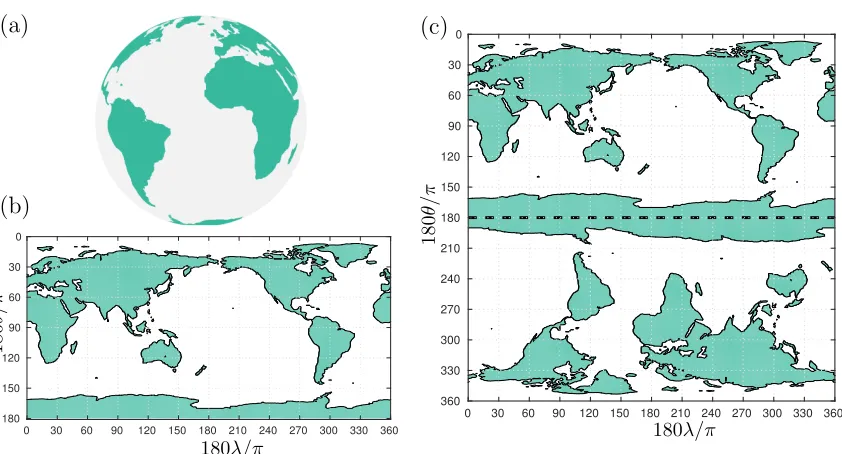
3.1 The DFS method applied to the globe. (a) An outline of the land
masses on the surface of earth. (b) The projection of the land masses
using latitude-longitude coordinates. (c) Land masses after applying
the DFS method, shown in extended coordinates with the dashed line
indicating the south pole. This is a BMC-I “function” that is periodic
in longitude and latitude. . . 29
3.2 Low rank approximants to a function on the sphere, ˜f = cos(1 + 2π(cosλsinθ + sinλsinθ) + 5 sin(πcosθ)), (λ, θ) ∈ [−π, π]2. Figures (a)-(d) are the respective rank 2, 4, 8, and 16 approximants to ˜f
constructed by the structure-preserving GE procedure in Section 3.2.
Figures (e)-(h) are the respective rank 2, 4, 8, and 16 approximants to
˜
fconstructed by the standard GE procedure [67], which is not designed to preserve the BMC-I structure. In figures (e) and (f), one can see
that a pole singularity is introduced when structure is not preserved. . . 30
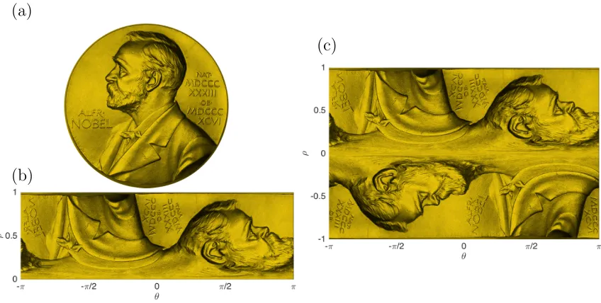
medal. (a) The medal. (b) The projection of the medal using polar
coordinates. (c) The medal after applying the disk analogue to the
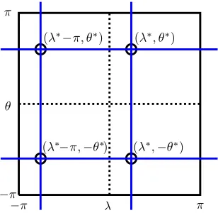
DFS method. This is a BMC-II “function” that is periodic in θ and defined over ρ∈[−1,1]. . . 31 3.4 The entries of the 2 × 2 GE pivot matrix (black circles), and the
corresponding row and column slices (blue lines) of ˜f containing these values. We only select pivots of this form during the GE procedure. . . . 32
3.5 A continuous idealization of our structure-preserving GE procedure on
BMC functions. In practice, we use a discretization of this procedure
and terminate it after a finite number of steps. . . 37
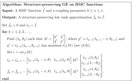
3.6 Left: The function f(x, y, z) = cos(xz − siny) on the unit sphere. Right: The “skeleton” used to approximate f that is found via the BMC structure-preserving GE procedure. The blue dots are the entries
of the 2×2 pivot matrices used by GE. The GE procedure only samples
f along the blue lines. The underlying tensor grid (in gray) shows the sampling grid required without low rank techniques, which cluster near
the poles. . . 38
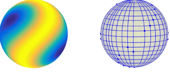
on the unit disk. Right: The adaptively selected skeleton for ˜g. The blue dots are the pivot locations selected via GE. The GE procedure
only samples g along the blue lines. The underlying tensor product grid (in gray) shows the sample points required to approximate g to approximately machine precision without the GE procedure applied to
the DFS method. The oversampling of the tensor grid, in contrast to
the low rank skeleton, can be seen. . . 39
3.8 A comparison of low rank approximations to the functions in (3.23)
computed using the SVD and the iterative GE procedure. TheL2error
is plotted against the rank of the approximants toφ1 and φ2. The L2
error given by the SVD approximants are optimal and we observe that
that the low rank approximants constructed by the GE procedure are
near-optimal. . . 52
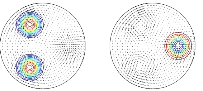
4.1 Arrows indicate the tangent vector field generated from u = ∇S ×ψ, whereψ(λ, θ) = cosθ+ (sinθ)4cosθcos(4λ), which is the stream func-tion for the Rossby–Haurwitz benchmark problem for the shallow water
wave equations [79]. After constructing ψ in Spherefun, the tangent vector field was computed using u = curl(psi), and plotted using
quiver(u). The superimposed false color plot represents the
vortic-ity of u and is computed using vort(u). . . 66
together with its curl, ∇ ×u (right), and divergence,∇ ·u (left). The field was plotted usingquiver(u), while the curl and divergence were
computed usingcurl(u)anddiv(u)respectively, and plotted using
contour. . . 75
5.1 Left: Solution to ∇2u = sin(50xyz) with a zero integral constraint computed by f = spherefun(@(x,y,z) sin(50*x.*y.*z));
u = spherefun.poisson(f,0,150,150);, which employs the
algorithm above with m = n = 150. Right: Execution time of the Poisson solver as a function of the number of unknowns, nm/2, when
m=n. . . 80 5.2 Left: Solution to ∇2u=g with boundary conditionu(θ,1) = 1, where
g is given in (5.17). Right: Execution (wall clock) time of the Poisson solver as a function of the number of unknowns,mn/2. We denote the degrees of freedom by mn/2 because this number is used to define the solutionu on the disk, where mn unknowns are used on ˜u. . . 86
discretization of the boundary value problem, ∂ u/∂x − xu = 0,
u(−1) = Ai(−p3
1/ε), u(1) = Ai(p3
1/ε), where ε = 1×10⁻⁵, and Ai are the Airy functions. This is called Airy’s equation. Here, n= 34 and there are 223 nonzero entries. The two dense upper rows are the
result of the boundary conditions. The final system used to compute
the solution to machine precision will be similarly sparse, but of size
n= 258. Right: The solution to the boundary value problem. The L2
norm of the error for the solution is O(10−14). . . 109
CHAPTER 1
INTRODUCTION
Polar and spherical geometries occupy a central role in scientific computing and
engineering, with applications in fluid dynamics [39, 55], optics [41], astrophysics [3,
11, 29, 51, 63], weather forecasting and climate modeling [17, 20, 25, 40, 45, 49, 59], and
geophysics [24,80]. Advances in these areas increasingly require accurate and effective
approximation methods for functions defined on the unit disk or the surface of the unit
sphere. To take advantage of convenient algorithms, coordinate transforms are often
applied that map functions in polar and spherical geometries to rectangular domains.
Unfortunately, this method has several significant drawbacks: it introduces one or
more artificial singularities into the problem, making smoothness over the poles of
the sphere (and origin of the disk) difficult to enforce. Interpolation schemes derived
from these mappings typically oversample the function near the singularities, and this
can severely hamper computational efficiency. Additionally, rectangular coordinate
transforms for functions on the sphere destroy the inherent bi-periodicity of such
functions, making the FFT inapplicable in one direction.
This thesis presents a new method for computing with functions in polar and
spherical geometries. By synthesizing a classic technique known as the double Fourier
sphere (DFS) method with a new structure-preserving Gaussian elimination
polar and spherical geometries are effectively overcome. This results in an efficient
and adaptive method of approximation for functions on the sphere and disk, with
approximants that enjoy a plurality of desirable attributes: 1) A structure that allows
the use of FFT-based algorithms in both variables, 2) smoothness over the poles of the
sphere (and origin of the disk), 3) stability for differentiation, and 4) an underlying
interpolation grid that rarely oversamples the function.
This approach is used to create an integrated computational framework for
work-ing with functions in polar and spherical settwork-ings, includwork-ing the development and
implementation of algorithms for integration, function evaluation, vector calculus,
and the solving of Poisson’s equation, among many other things. These ideas are
implemented in a software package that is publicly available through the open-source
Chebfun software system, which is written in MATLAB [21]. This development allows
investigators to compute on the sphere and disk without concern for the underlying
discretization or procedural details, providing an intuitive platform for data-driven
computations, explorations, and visualizations, all occurring at an accuracy near
machine precision.
This thesis is organized as follows: A review of global polynomial and
trigono-metric interpolation methods in the 1D setting is given in Section 2.1, as this forms
a basis for our approach. The concept of low rank approximation for 2D functions is
reviewed in Section 2.2, followed by an overview of existing methods of approximation
for functions on the sphere (see Section 2.3) and the disk (see Section 2.4).
In Chapter 3, a classic procedure known as the double Fourier sphere (DFS)
method, as well as its disk analogue, are used to introduce the concept of
block-mirror-centrosymmetric (BMC) structure (see Section 3.1). A new, BMC
method is used to construct low rank approximations to functions on the sphere and
the disk. The relationship between this GE procedure, BMC structure, and parity
properties of functions in polar and spherical geometries is discussed in Section 3.4.
Section 3.5 provides theoretical results related to convergence of the GE procedure,
and this is followed by a discussion of near-optimal convergence behaviors observed
in practice (see Section 3.6).
Chapter 4 describes a collection of algorithms for computing on the sphere (see
Section 4.2) and disk (see Section 4.3) through the use of low rank approximations.
These algorithms have been implemented in the Chebfun computing system and are
available for exploration at www.chebfun.org.
Chapter 5 applies the DFS method in conjunction with Fourier and
ultraspher-ical spectral methods to develop optimal Poisson solvers for both the sphere (see
Section 5.1) and the disk (see Section 5.2).
Appendix A offers a collection of observations on the properties of BMC functions,
including a discussion of linear algebra related to discretizations of BMC functions
(see Section A.1), and a derivation of the SVD for BMC functions (see Section A.2).
Appendix B provides an overview of the ultraspherical spectral method, which is used
to formulate a Poisson solver on the disk.
Author Contributions and Related Publications
This thesis is the result of the collective efforts of myself, Prof. Grady Wright (Boise
State Univ.), and Prof. Alex Townsend (MIT). Results related to the sphere and
the initial conception of BMC structure-preserving GE were largely collaborative.
disk, developed the algorithms for numerically computing with functions on the disk,
and created the Diskfun software. I was also the lead author of our paper about
numerical computing with functions on the disk [71]. While writing this thesis and
working closely with my advisors, I additionally developed several new results and
observations that apply to functions on the sphere and the disk. This includes
a proof that the BMC structure-preserving GE procedure in Chapter 3 converges
geometrically (see Section 3.5), an explicit formulation and formal proof that the GE
algorithm preserves BMC structure (see Section 3.2), and an explicit description of
precisely why approximants that have BMC structure are differentiable on the sphere
and disk (see Sections 4.2.4 and 4.3.4).
Overall, two papers related to this research have been produced [70, 71]; this work
complements these papers by providing additional insights, results, and examples.
This includes an extended discussion of key notions from approximation theory and
alternate methods of approximation in polar and spherical geometries in Chapter 2,
new results related to the convergence properties of the GE algorithm and parity
properties associated with BMC functions in Chapter 3, the development of aweighted
SVD algorithm for functions on the sphere, as well as additional details concerning
differentiation on the sphere in Chapter 4, and an extended description of a highly
optimized Poisson solver for the disk in Chapter 5. These insights are supplemented
by additional materials contained in the appendices, including observations on BMC
matrices and an explicit derivation of the SVD for BMC functions (Appendix A), and
CHAPTER 2
BACKGROUND
In [4], global polynomial interpolants are used to create a framework for numerically
computing with 1D functions, and this idea is extended to periodic 1D functions in [81]
through the use of trigonometric interpolants. These ideas are implemented within
the software system Chebfun. The extension of these ideas to 2D is presented in [67],
and in this thesis, we develop an analogous approximation method for computing
with functions on the sphere and disk. Using this method, many operations on
bivariate functions can be performed through essentially 1D procedures involving
univariate Fourier and Chebyshev expansions. This makes the method especially
amenable to implementation within Chebfun, where highly optimized algorithms for
a range of operations involving 1D functions are available. We have implemented our
approximation method and the associated algorithms in the Spherefun and Diskfun
software systems, which are available as an integrated part of Chebfun.
Our approximation method requires the use of global polynomial and
trigonomet-ric interpolants to 1D functions, and relies on the convergence properties associated
with these interpolants (see Section 2.1). We also use recent developments in low
rank approximation methods for 2D functions (see Section 2.2.2), and classic
tech-niques associated with numerically representing functions on the sphere and disk (see
also gives a broad overview of alternative techniques currently used for computing
with functions in polar and spherical geometries.
2.1
1D Function Approximation
2.1.1 Trigonometric Polynomial Interpolation
For approximations to functions on the sphere and disk, we will require the use
of interpolants for periodic functions on [−π, π]. Let f : [−π, π] → C be a 2π -periodic function that is Lipschitz continuous. Then, f has a unique Fourier series that converges absolutely and uniformly:
f(x) =
∞ X k=−∞
˜
ckeikx, x∈[−π, π], (2.1)
where ˜ck = 21πR−ππf(x)e−ikxdx are the Fourier coefficients of f. Truncating (2.1) gives an approximation to f:
fm(x) =
m X k=−m
˜
ckeikx, x∈[−π, π]. (2.2)
The functionfmis a trigonometric polynomial of degreem, referred to as the degreem
Fourier projection of f. To compute (2.2), we can approximate the integrals defining
each ˜ck by using the trapezoidal rule with the following 2m+ 1 quadrature points:
xk =−π+ 2kπ
2m+ 1, 0≤k ≤2m. (2.3)
However, as described in [81], this is equivalent to interpolating f at the points given in (2.3) with the basis functions {eikx} . This finds pm(x), the trigonometric
interpolant to f of degree m, which can be written as
pm(x) =
m X k=−m
The coefficients{ck}and{c˜k}are related to one-another through analiasing formula, so that theoretical results for (2.2) have analogous interpretations for (2.4) [81]. This
is useful because (2.2) is convenient for analytical work, but it is easier numerically
to use (2.4). Here, we list key convergence properties for pm (see [81] and [72] for related results on fm). The first result is related to the bounded total variation of a function, defined as follows:
Definition 2.1 (Bounded total variation). A function f(x), x ∈ [a, b] is said to be
of V bounded total variation if
V =
Z b a
|f0(x)|dx <∞.
This notion can be used to understand the rate of convergence for trigonometric
interpolants of differentiable functions. In the following theorems,||·||∞is the infinity
norm, i.e., ||f||∞ = sup{|f(x)|:x∈[−π, π]}.
Theorem 2.1 (Convergence for differentiable periodic functions). For ν ≥ 1, let f
be ν times differentiable, 2π-periodic function on the interval [−π, π], with f(ν) of
bounded total variation V. Let pm be the degree m trigonometric interpolant of f as
in (2.4). Then, for m≥ν,
||f−pm||∞≤
2V πνmν,
i.e., ||f −pm||∞ =O(m −ν
).
If f is analytic, convergence depends on the region for which f is analytically continuable in the complex plane.
|f(z)| ≤M in an open strip of half-width α > 0 around the real axis in the complex
z-plane, then
||f−pm||∞≤
4M e−αm eα−1 ,
i.e., ||f−pm||∞ =O(e−αm).
The proofs for these theorems are given in [81], and rely on related theorems
about the rates of decay of the coefficients in (2.4). These theorems state specific
results associated with a general maxim in approximation theory: the smoother
a function is, the faster its approximants converge. Trigonometric interpolants to
periodic functions that are ν-times differentiable (with a νth derivative of bounded total variation) converge at algebraic rates. Interpolants to functions that are analytic
converge at geometric rates, and interpolants to functions that are entire converge
super-geometrically. Thus, for sufficiently smooth periodic functions, trigonometric
interpolation offers an excellent method of approximation.
Henrici describes a procedure for evaluating pm at any point x∗ ∈[−π, π] in only
O(N) operations [35], whereN = 2m+1 is the number of interpolation points in (2.3). Alternatively, pm can be uniquely represented by the set of coefficients {ck}mk=−m.
Given the values of f(xk) at each xk in (2.3), the FFT finds {ck}mk=−m in only O(NlogN) operations. Likewise, if {ck}mk=−m are known, the inverse FFT provides
an efficient way to sample f, givings its values at each xk in (2.3) in O(NlogN)
operations.
2.1.2 Chebyshev Polynomial Interpolation
For numerically representing functions on the disk, we require approximations to
Im(
z
)
Re(z)
Figure 2.1: The (2n)th roots of unity for n = 16 are plotted on the unit circle. Their projection to the real axis results in the Chebyshev points (red) on the interval [−1,1].
Let f : [−1,1]→C be any continuous function. Without the assumption of peri-odicity, interpolants to f at equally-spaced points over [−1,1] become exponentially ill-conditioned, with interpolants at n points potentially producing numerical errors of sizeO(2n), even in cases wheref is analytic on [−1,1] [74, Ch. 13]. For this reason, we seek an alternate set of interpolation points.
Consider the set of n+ 1 equally-spaced angles {θk}kn=0, θk∈[0, π]. These angles
are the arguments for the (2n)th roots of unity {zk =eikπ/n}nk=0. The points
xk = Re(zk) are called the Chebyshev points, and can be expressed conveniently as
xk=−cos
kπ n
, 0≤k ≤n. (2.5)
Interpolating f at the n + 1 Chebyshev points gives an approximation to f that is closely related to the expansion of f in the Chebyshev polynomial basis. The Chebyshev polynomial of degree n is defined as
Tn(x) = cos(nθ), θ = cos −1
(x), x∈[−1,1].
< Tm, Tn>w= 2
π
Z 1 −1
Tm(x)Tn(x)
p
1−x2
=
2, m=n= 0,
1, m=n, m, n6= 0 0, m6=n.
(2.6)
These polynomials form a complete basis for functions on [−1,1] that are square-integrable with respect to (2.6), and for such a function f, there exists a unique series
f(x) =
∞ X k=0
˜
akTk(x), x∈[−1,1], (2.7)
that converges absolutely and uniformly to f. Truncating this series to n+ 1 terms forms the approximantfn, known as the degreen Chebyshevprojection off. As with trigonometric polynomial approximation, it can be more convenient computationally
to consider the unique interpolant to f at the n+ 1 Chebyshev points:
pn(x) = n X k=0
akTk(x), x∈[−1,1]. (2.8)
Here, each ak is related to ˜ak through an aliasing formula [74], and theoretical results forfn correspond closely to results forpn. Chebyshev interpolants are known to have
very good convergence properties for functions with some degree of smoothness, and
we give two essential results here.
Theorem 2.3 (Convergence for differentiable functions). Let f be ν ≥ 1 times differentiable on [−1,1] with f(ν) of bounded variation V. If pn is the degree n
Chebyshev interpolant of f given by (2.8), then for any n≥ν,
||f −pn||∞≤
4V πν(n−ν)ν,
i.e., ||f−pn||∞=O(n −ν
).
Iff is analytic on [−1,1], the rate of convergence depends on the region for which
Im(
z
)
Re(z)
Figure 2.2: Berstein ellipses of increasing size. The ellipses correspond to the respective parametersρ= 1.1,1.2, . . .1.8,2, with innermost ellipse havingρ= 1.1.
ellipses, defined below.
Definition 2.2 (Berstein ellipse). The Berstein ellipseEρ, ρ >1, is the open region
of the complex plane bounded by an ellipse with foci at ±1 and a semimajor and
semiminor axis that sum to ρ.
Figure 2.2 displays Berstein ellipses for several choices ofρ. Using Berstein ellipses, we can precisely describe the convergence behavior of Chebyshev interpolants to
analytic functions.
Theorem 2.4 (Convergence for analytic functions). Let f be analytic on [−1,1]
and analytically continuable to the Berstein ellipse Eρ, satisfying |f| < M for some
constant M >0. If pn is the degree n Chebyshev interpolant tof, then
||f−pn||∞ ≤
4M ρ−n ρ−1 ,
i.e., ||f−pn||∞=O(ρ −n
).
Proofs of Theorems 2.3 and 2.4 can be found in [74]. These theorems show that
properties. In fact, Chebyshev interpolants offer a near-best approximation for
con-tinuous functions. In [74, Ch. 16], it is shown that if f is continuous on [−1,1] and
p∗n is the best degree n polynomial approximation to f with respect to the infinity
norm, then
||f−pn||∞≤
2
πlog(n+ 1) + 2
||f −p∗n||∞.
This inequality states that the difference between the best approximation tof and the Chebyshev interpolant to f is at maximum O(logn). Asymptotically, one cannot do better than this: it is shown in [12] that for any setSofn+1 distinct points on [−1,1], there always exists a continuous function f such that the polynomial interpolant p†n
tof onS satisfies
||f −p†n||∞ ≥ 1.52125 +
2
πlog(n+ 1)
||f −p∗n||∞.
It is in this sense that Chebyshev interpolants offer a near-best approximation to f, and this idea is made precise in [74, Ch. 15].
Chebyshev interpolants possess one more important quality: Given the values of
f at the n+ 1 Chebyshev points, the coefficients in (2.8) can be computed through the fast cosine transform in only O(nlogn) operations. The inverse of this operation also costs only O(nlogn) operations, providing a convenient way to sample f when the coefficients in (2.8) are known.
2.2
Low Rank Approximation for 2D Functions
In [67], a general approach for computing with 2D functions over a bounded
use this idea in Chapter 3 to develop a low rank approximation method for functions
in spherical and polar geometries. Here, we review the concepts from [67].
Let f(x, y) be a bivariate function on [−1,1]2, and note that any function on a more generalized rectangular domain can be mapped to [−1,1]2 by a change of variables. A nonzero function f is called a rank 1 function if it can be written as a product of two univariate functions, i.e., f(x, y) =c(y)r(x). A function is of at most rank K if it can be written as a sum of K rank 1 functions. While most functions are mathematically of infinite rank, smooth functions can typically be approximated
to machine precision by a rank K truncation, i.e.,
f(x, y)≈
K X
j=1
cj(y)rj(x)
| {z }
fK
, (2.9)
for some relatively small K [64]. In practice, we are interested in thenumerical rank
of f. This is the minimum rank required to approximate f within some tolerance, such as machine epsilon, using any bounded function on [−1,1]2 of finite rank. For a prescribed value >0, this is given by
k = min{K ∈N: inf fK
||f−fK||∞ ≤||f||∞},
where the inner infimum is taken over the set of bounded rank K functions on [−1,1]2 [64].
The primary advantage of using low rank approximations is evident in [67] and
in Chapter 4 of this thesis, where several algorithms are devised that exploit the
low rank form in order to use highly efficient 1D procedures. To use this form of
approximation effectively, several questions are in order: (1) Can every function be
constructing low rank approximations to an arbitrary function? (3) What are the
convergence properties of low rank approximations to functions? We will additionally
be concerned with whether an adaptive low rank approximation method can be
developed that preserves inherent geometric features of functions defined in polar
and spherical geometries.
2.2.1 The Singular Value Decomposition
We examine questions (1)-(3) by considering the best rank K approximation to f. For the L2 norm, this is given by thesingular value decomposition (SVD), also called the Karhunen–Lo`eve expansion, for bivariate functions [53]. It is shown in [33] that
if f is Lipschitz continuous in both variables, then the SVD converges absolutely and uniformly tof. Then,f is expressed by
f(x, y) =
∞ X
j=1
σjuj(y)vj(x), (x, y)∈[−1,1]2. (2.10)
Here, the singular values {σj} ∞
j=1 are non-negative, real, nonincreasing, and
limk→∞σk → 0. The sets of continuous singular functions, {uj} ∞
j=1 and {vj} ∞ j=1, are
each orthonormal with respect to the L2 inner product on [−1,1]. Furthermore, the set {σj} is uniquely determined for f, and the singular functions corresponding to each simple σj are unique up to complex signs.
In [53], it is shown that the best rank K approximation to f in the L2 norm is formed by truncating (2.10) to K terms. For this reason, the SVD is said to provide an optimal rank K approximation to f. In [69], it is shown that properties of convergence for the SVD are linked to the smoothness of the function. Given any
the rank K truncation of the SVD of f, then the error ||f −fK||∞ decays at the rate of O(K−ν). If all f(x∗, y) are analytically continuable to a Bernstein ellipse of parameter ρ in the complex plane that contains the interval [−1,1], then ||f−fk||∞
decays at a geometric rate prescribed by ρ [69].
For such functions, the continuous SVD can be explicitly constructed by first
performing the continuous analogue to LU factorization on f, and then performing a QR factorization the resulting quasimatrices [69]. Alternatively, one could samplef
and numerically compute the SVD of the resulting matrix using standard techniques.
The cost of computing the SVD is O(N3) operations, where N is the number of samples required to resolvef to a specified tolerance in both x and y.
The SVD shows us that at least one method of low rank approximation exists for
a large class of functions. The approximants have very good convergence properties,
but they are computationally expensive to construct. For this reason, we seek an
alternative technique.
2.2.2 Iterative Gaussian Elimination on Functions
Given a matrixAof rankn,K < nsteps of Gaussian elimination (GE) with complete or rook pivoting can be used to construct a near-best rank K approximation to A, provided that the singular values of A decay sufficiently fast [28]. Using a variety of pivoting strategies, methods such as adaptive cross approximation [6], two-sided
interpolative decomposition [32], and Geddes–Newton approximation [16] apply GE
in the continuous setting to create low rank approximations to functions. In [67],
an adaptive, iterative variant of GE with complete pivoting is used to develop a
procedure for approximating functions in polar and spherical geometries is based on
an extension of this idea (see Chapter 3).
Standard GE on a matrix A with complete pivoting proceeds by choosing the entry with the maximal absolute value, A(i, j), as a pivot. At each GE step, a rank 1 matrix is formed from this pivot and subtracted fromA:
A ←A−A(:, j)A(i,:)/A(i, j),
where A(:, j) is jth column of A, and A(i,:) is the ith row of A. This step zeros out the row and column containing the pivot and also reduces the rank ofA by one. The resulting matrix is called the residual. The process is then repeated on the residual,
and the algorithm proceeds until the residual is the zero matrix. Summing the first
K rank 1 matrices formed within this process provides a rank K approximation to
A.
In a similar way, given a function f(x, y), denote the maximum absolute value of
f for (x, y)∈[−1,1]2 as f(x∗, y∗). Replacing A with f, the GE step is given by
f(x, y) ←− f(x, y)− f(x
∗
, y)f(x, y∗)
f(x∗, y∗)
| {z }
A rank 1 approx. tof
. (2.11)
In this scheme, the functionsf(x∗, y) are referred to as “column slices” off. Similarly,
f(x, y∗) are “row slices.” As with GE on matrices, the GE step produces a residual such that f(x∗, y) = f(x, y∗) = 0. Unlike a matrix, f is typically of infinite rank, so the GE procedure is terminated after the absolute maximum of the residual falls
below some specified relative tolerance, such as the product of machine epsilon and
the (approximate) maximum value of the function. The number of steps required to
achieve this is an upper bound on the numerical rank1 of f, and as discussed in [64],
1
smooth functions are typically of low numerical rank.
Each time we apply a GE step to f, a rank 1 function is selected. AfterK steps, we can collect these rank 1 functions and construct a rank K approximation tof:
f(x, y)≈
K X
j=1
djcj(y)rj(x). (2.12)
Here, dj is a coefficient derived from the jth pivot, and cj(y) and rj(x) are the
jth column and row slices, respectively, selected during the GE procedure. The computational cost of performing K steps of GE on f is O(K3). Each univariate function in (2.12) is then adaptively resolved in O(K2(m+n)) operations, where m
and n are the maximum number of samples required to resolve each cj(y) and rj(x), respectively [67].
In [64], it is shown that this GE procedure is a near-optimal and highly efficient
method for approximating 2D functions in standard rectangular domains. We now
turn to the specific challenges associated with numerically representing functions in
polar and spherical geometries.
2.3
Existing Approximation Methods for Functions on the
Sphere
To numerically represent 2D functions that are defined on the surface of the unit
sphere, it is convenient to relate computations with functions on the sphere to
func-tions defined over a rectangular domain. Given a function f(x, y, z) in Cartesian coordinates, the spherical coordinate transform is given by
where λ is the azimuth angle and θ is the polar (or zenith) angle (measured from the north pole). This change of variables allows one to compute with the function
f(λ, θ), as opposed to f(x, y, z) restricted to the surface of the sphere.
Unfortunately, this transform introduces artificial singularities at the north and
south poles, since, by (2.13), for all λ ∈ [−π, π], (λ,0) maps to (0,0,1), and (λ, π) maps to (0,0,−1). Furthermore, the mapping does not preserve the natural periodic-ity off in the latitude direction. The introduced singularities act as north and south boundaries on the rectangle, making smoothness over the poles difficult to enforce.
This mapping is also problematic for interpolation schemes, as it results in grids on
the sphere that are severely and redundantly clustered near the poles.
The approach we develop in Ch. 3 resolves these issues. Through the use of
the double Fourier sphere (DFS) method (see Section 3.1), the periodicity of f in θ
is recovered. We combine this scheme with a new, structure-preserving low rank
approximation method, and this mitigates the unphysical effects of the artificial
singularities, as well as issues associated with oversampling f near the poles. Below, we review some alternative techniques for computing on the sphere in order to put
our new method in context.
2.3.1 Spherical Harmonic Expansions
Spherical harmonics are an appealing choice for representing functions on the surface
of the sphere [2, Chap. 2] because they are analogous to trigonometric expansions
for periodic functions. They have been used extensively and effectively in weather
forecasting [20, Sec. 4.3.2], least-squares filtering [37], and for finding the numerical
solution of separable elliptic equations. The truncated spherical harmonic expansion
f(λ, θ)≈
N X
`=0 ` X m=−`
c`,mY`m(λ, θ), (2.14)
whereY`mis the spherical harmonic function with degree`and orderm[47, Sec. 14.30],
and
c`,m =
Z 2π 0
Z π 0
Y`m(λ, θ)f(λ, θ) sinθ dθ dλ.
The truncated expansion (2.14) provides essentially uniform resolution of f over the sphere. The coefficients 0 ≤ ` ≤ N and c`,m for −` ≤ m ≤ ` in (2.14) can be approximated with a discrete spherical harmonic transform, and there are fast
O(N2logN) complexity algorithms available for these transforms [46, 76]. However, highly adaptive discretizations are computationally unfeasible in this setting due to
a high preprocessing cost associated with these algorithms. In our setting, fast and
highly optimized algorithms are more readily available via the FFT.
2.3.2 Quasi-isotropic Grid-based Methods
Quasi-isotropic grid-based methods, such as those that use the “cubed-sphere”
(“quad-sphere”) [52, 62], geodesic (icosahedral) grids [5], or equal area “pixelations” [31],
partition the sphere into (spherical) quads, triangles, or other polyhedra. This avoids
introducing artificial singularities and results in far less oversampling of functions
compared to grids designed by standard coordinate transforms. They are particularly
useful for computations in which 3-5 digits of accuracy are sought and they are also
highly amendable to parallelization. However, for 8-15 digits of accuracy, sample
points usually become clustered along the artificial boundaries associated with these
grids. Our GE procedure takes function samples that are adaptively selected during
tensor product of 1D uniform grids (see Figure 3.6) that only cluster if the function
itself requires it.
2.3.3 Radial Basis Functions
Radial basis functions (RBFs), or spherical basis functions [23], allow one to place
sampling points at any location on the sphere. This is highly advantageous as
sampling can be tailored to capture a function’s features of interest, and these
meth-ods have been successfully applied in numerical weather prediction and solid earth
geophysics calculations [24, 80].
While spectral accuracy is possible with these methods, the state-of-the-art
al-gorithms have a computational complexity that grows cubically in the total degrees
of freedom [27]. Consequently, these methods are currently too costly for general
purpose computations with functions on the sphere.
2.3.4 The Double Fourier Sphere Method
The double Fourier sphere (DFS) method is a technique that can be used to recover
the periodicity of the sphere in the latitude direction [45]. This method forms one
of the pillars of our new approximation technique, so we hold off reviewing it until
Chapter 3.
2.4
Existing Approximation Methods for Functions on the
Disk
x=ρcosθ, y=ρsinθ, (θ, ρ)∈[−π, π]×[0,1]. (2.15)
This relates a function on the disk to a function defined over a rectangular domain,
where more convenient algorithms can be applied. Unfortunately, this transform
introduces an artificial singularity and unphysical boundary at ρ = 0. One solution involves expanding g(θ, ρ) in a basis that inherently enforces smoothness over ρ= 0, but such basis choices are not associated with fast transforms.
Unsatisfied with choosing between the use of fast algorithms and smoothness at the
origin, we present an efficient method in Chapter 3 that prioritizes both. We expandg
in the Fourier–Chebyshev basis so that fast, FFT-based algorithms are applicable, but
combine an analogue of the DFS method (see Section 3.1) with a structure-preserving
Gaussian elimination (GE) procedure to enforce that approximants are smooth over
the origin. Below, we offer a brief discussion of alternative strategies.
2.4.1 Radial Basis Functions
As a mesh-free method, radial basis functions are useful for applications on a variety of
geometries, such as the sphere and disk [26] (for more discussion, see Section 2.3.3).
In [36] and [38], an algorithm for approximations on the disk is developed that
arranges interpolation points so that the computational cost of the method reduces
from O(N3) to O(NlogN) operations, where N is the number of function samples taken. Unfortunately, ill-conditioning prevents this method from reaching machine
2.4.2 Conformal Mapping
Using the inverse of the cosine leminiscate function, a function g on the unit disk can be mapped conformally to the unit square [1, 54]. This allows g to be expressed as a bivariate Chebyshev expansion so that FFT-based transforms are applicable.
Unfortunately, the mapping introduces four artificial singularities corresponding
to the corners of the unit square. Interpolation grids based on this scheme are
unneces-sarily redundant near these singularities, and this adversely affects the computational
efficiency gained from use of the FFT. In contrast, our approach also enables the use of
FFT-based transforms, but we combine this with an adaptive low rank approximation
procedure that does not oversample the function.
2.4.3 Basis Expansions
Observing in (2.15) that g is periodic in θ, an approximation to g can be obtained from a Fourier expansion in θ:
g(θ, ρ)≈
m/2−1 X k=−m/2
φk(ρ)e ikθ
, (θ, ρ)∈[−π, π]×[0,1], (2.16)
where we assume m is an even integer2 and φk(ρ) is a function to be selected. The most appropriate basis for expanding φk(ρ) is not immediately obvious. Below, we discuss three of the most common choices.
2.4.3.1 Cylindrical Harmonic Expansions
Cylindrical harmonics are the natural analogue of the spherical harmonics, as they
are the eigenfunctions of the Laplace operator in cylindrical coordinates at a fixed
2
height [19]. If g is sufficiently smooth and satisfies g(θ,1) = 0, an approximation to
g is given by
g(θ, ρ)≈
m/2−1 X k=−m/2
n−1 X j=0
ajkJk(ωkjρ)eikθ, (θ, ρ)∈[−π, π]×[0,1], (2.17)
where Jk is the kth order Bessel function, and ωkj is the jth positive root of Jk [19, Ch. 9]. This expansion can also be modified to include a inhomogeneous boundary
condition. For (2.16) to be infinitely differentiable, each φk(ρ) must decay like ρ k
or
faster near ρ = 0. The cylindrical harmonics are attractive because they inherently satisfy this condition. However, there is no readily available fast transform for
computing the coefficients in (2.17), and for this reason, we do not use cylindrical
harmonics in our approach.
2.4.3.2 One-sided Jacobi Polynomial Expansions
Expressingφk(ρ) with one-sided Jacobi polynomials results in an expansion ofg(θ, ρ) in the Zernike polynomial basis, Zjk(θ, ρ) [10, 78]. This set of polynomials is con-sidered theoretically analogous to the Legendre polynomials due to its orthogonality
properties [7]. Using this expansion,
g(θ, ρ)≈
m/2−1 X k=−m/2
n−1 X j=0
ajkρ |k|
Pj(0,k)(2ρ2−1)eikθ, (2.18)
where Pj(0,k) is the Jacobi polynomial of degree j with parameters (0, k). Terms in this expansion inherently satisfy smoothness conditions because they include a
kth order zero at ρ = 0. The Zernike polynomials are often considered the basis of choice for approximation on the disk, and have been used to develop a method
that results in sparse operators for solving the Helmholtz and Poisson equations [44].
been developed to capture the regularity of vector- and tensor-valued functions on
the disk [77].
The primary disadvantage of using the one-sided Jacobi polynomials is the lack of
a fast transform for computing the coefficients in (2.18). Since our approach relies on
an interpolative, data-driven and adaptive scheme, we require fast transforms, and
therefore do not make use of one-sided Jacobi expansions.
2.4.3.3 Fourier–Chebyshev Expansions
Expandingφk(ρ) in the Chebyshev basis gives the Fourier–Chebyshev approximation tog:
g(θ, ρ)≈
m/2−1 X k=−m/2
n−1 X j=0
ajkTj(2ρ−1)eikθ, (θ, ρ)∈[−π, π]×[0,1], (2.19)
where Tj(·) is the degree j Chebyshev polynomial defined on [−1,1]. By sampling
g on an n × m Fourier–Chebyshev tensor product grid, the coefficients in (2.19) can be found in only O(mnlog(mn)) using FFT-based algorithms. Problematically, this choice does not naturally impose smoothness over the origin, and grids based
on this expansion unnaturally cluster near ρ = 0 [25]. Our approach resolves these drawbacks by combining the disk analogue to the DFS with a structure-preserving
low rank construction procedure (see Chapter 3).
2.4.4 The Disk Analogue to the Double Fourier Sphere Method
There are several spectral collocation schemes involving Fourier–Chebyshev grids that
alleviate the induced overresolution near ρ= 0 by double-sampling g so that
action is analogous to the DFS method. As it forms a crucial component of our new
CHAPTER 3
LOW RANK APPROXIMATION OF FUNCTIONS IN
SPHERICAL AND POLAR GEOMETRIES
In this chapter, we develop a new method for approximating functions on the sphere
and disk. The double Fourier sphere (DFS) method (see Section 3.1) is applied to
a function defined on the sphere or disk, and this introduces a crucial symmetry
structure related to the geometry of the domain. In Section 3.2, we develop a variant
of GE that generates low rank approximants while exactly preserving this structure,
and in Sections 3.3-3.6, we analyze several features of the new GE procedure. This
new method results in approximants with several desirable properties that can be
exploited to create highly efficient algorithms (see Chapter 4).
We will begin by considering functions defined on the unit sphere. Each
obser-vation we make has an analogous interpretation for functions defined on the disk.
At certain points in the chapter, it is more convenient to generalize by discussing a
broader class of functions that is inclusive of functions on the sphere or disk.
3.1
Intrinsic Structures for Functions on the Sphere and Disk
Merilees [45] observed that a simple technique can be used to transform a function
on the surface of the sphere to one on a rectangular domain while simultaneously
directions. This idea, known as the double Fourier sphere (DFS) method, was
developed further by Orszag [49], Boyd [8], Yee [82], Fornberg [25], and Cheong [17].
Transforming f(x, y, z) on the sphere to a function f(λ, θ) in spherical coordinates using (2.13) yields
f(λ, θ) = f(cosλsinθ,sinλsinθ,cosθ), (λ, θ)∈[−π, π]×[0, π].
With this transformation, the periodicity in the latitude direction has been lost. The
DFS method proceeds by “doubling up” the function to form an extension of f on (λ, θ)∈[−π, π]×[−π, π]. The extension is given by
˜
f(λ, θ) =
p(λ+π, θ), (λ, θ)∈[−π,0]×[0, π], q(λ, θ), (λ, θ)∈[0, π]×[0, π], p(λ,−θ), (λ, θ)∈[0, π]×[−π,0], q(λ+π,−θ), (λ, θ)∈[−π,0]×[−π,0],
(3.1)
where p(λ, θ) = f(λ −π, θ) and q(λ, θ) = f(λ, θ) for (λ, θ) ∈ [0, π]× [0, π]. The function ˜f is 2π-periodic in λ and θ, and is constant along the lines θ = 0 and
θ =±π, corresponding to the poles. With a slight abuse of notation, we depict ˜f as
˜
f =
"
p q
flip(q) flip(p)
#
, (3.2)
whereflip refers to the MATLAB command that reverses the order of the rows of a
matrix. The extension (3.1) is also called a glide reflection in group theory [42, §8.1].
As depicted in Figure 3.1 and seen in (3.2), the extended function ˜f has a structure close to a 2×2 centrosymmetric matrix, except that the last block row is flipped (mirrored). For this reason, we say that ˜f in (3.1) has a block-mirror-centrosymmetric (BMC) structure. This is formally defined as follows:
Definition 3.1. (Block-mirror-centrosymmetric functions) Leta, b∈R+. A function
˜
are functions p, q : [0, a]×[0, b] →C such that
˜
f(ξ, η) =
p(ξ+a, η), (ξ, η)∈[−a,0]×[0, b], q(ξ, η), (ξ, η)∈[0, a]×[0, b], p(ξ,−η), (ξ, η)∈[0, a]×[−b,0], q(ξ+a,−η), (ξ, η)∈[−a,0]×[−b,0].
(3.3)
Using (3.1), every continuous function on the sphere can be extended to a
continu-ous BMC function defined on [−π, π]×[−π, π] that is 2π-periodic (bi-periodic) in both variables. However, the converse is not true. It is possible to have a continuous BMC
function that is bi-periodic but is not constant at the poles, i.e., along the linesθ = 0 and θ =π, and therefore is not associated with a continuous function on the sphere. For example, the function f(λ, θ) = cos(2θ) cos(2λ) is a bi-periodic BMC function, but it is not constant when θ = 0 or θ = π. We capture this important aspect of BMC functions created through the DFS method with the following definition:
Definition 3.2 (BMC-I functions). A function f˜: [−a, a]×[−b, b]→C is a Type-I BMC (BMC-I) function if it is a BMC function, and additionally, there are constants
C1 and C2 such that f(·,0) =C1 and f(·,±b) =C2.
By operating on the BMC-I function ˜f, we can incorporate a structure associated with the sphere into our computations and relate the result back tof. It is fundamen-tal that any approximant to ˜f possess BMC-I structure, and the structure-preserving GE procedure in Section 3.2 is designed with this in mind. Figure 3.2 illustrates the
importance of this fact: pole singularities are introduced when the approximation
strategy does not enforce BMC-I structure, and this reduces accuracy in subsequent
computations, such as differentiation.
The DFS method can also be applied to functions on the disk. Consider the
0 30 60 90 120 150 180 210 240 270 300 330 360 0 30 60 90 120 150 180 (a) (b) 180λ/π 180 θ/π
0 30 60 90 120 150 180 210 240 270 300 330 360 0 30 60 90 120 150 180 210 240 270 300 330 360 (c) 180λ/π 180 θ/π
Figure 3.1: The DFS method applied to the globe. (a) An outline of the land masses on the surface of earth. (b) The projection of the land masses using latitude-longitude coordinates. (c) Land masses after applying the DFS method, shown in extended coordinates with the dashed line indicating the south pole. This is a BMC-I “function” that is periodic in longitude and latitude.
boundary at ρ = 0 (see Section 2.4). By expanding the domain of ρ from [0,1] to [−1,1], g can be extended to form a new function, ˜g : [−π, π]×[−1,1]→C, so that
ρ = 0 is no longer treated as a boundary. Mathematically, this extension of g can be expressed via functions p(θ, ρ) and q(θ, ρ), (θ, ρ) ∈ [0, π]×[0,1]. The extended function ˜g is given by
˜
g(θ, ρ) =
q(θ+π, ρ), (θ, ρ)∈[−π,0]×[0,1], p(θ, ρ), (θ, ρ)∈[0, π]×[0,1], q(θ,−ρ), (θ, ρ)∈[0, π]×[−1,0], p(θ+π,−ρ), (θ, ρ)∈[−π,0]×[−1,0],
(3.4)
and we observe in (3.4) that ˜g also possesses BMC symmetry (see Def. 3.3). This idea is conceptually analogous to the DFS method, although the original motivations for
(a) (b) (c) (d)
(e) (f) (g) (h)
Figure 3.2: Low rank approximants to a function on the sphere, ˜f = cos(1 + 2π(cosλsinθ+ sinλsinθ) + 5 sin(πcosθ)), (λ, θ) ∈[−π, π]2. Figures (a)-(d) are the respective rank 2, 4, 8, and 16 approximants to ˜f constructed by the structure-preserving GE procedure in Section 3.2. Figures (e)-(h) are the respective rank 2, 4, 8, and 16 approximants to ˜f constructed by the standard GE procedure [67], which is not designed to preserve the BMC-I structure. In figures (e) and (f), one can see that a pole singularity is introduced when structure is not preserved.
to alleviate excessive grid clustering near ρ = 0 in Fourier–Chebyshev interpolation schemes [22, 25], and several variants have been proposed [10, 34].
Figure 3.3 depicts the disk analogue to the DFS method applied to the Nobel
Prize medal. In addition to having BMC structure, ˜g must be constant along the line ρ = 0. This feature of ˜g is not shared by all BMC functions, but it is a crucial property of BMC functions associated with the disk. For this reason, we define a
second variant of BMC functions:
Definition 3.3 (BMC-II function). A function ˜g : [−a, a]×[−b, b]→C is a Type-II
BMC (BMC-II) function if it is a BMC function and g(·,0) = constant.
(b)
(c)
Figure 3.3: The disk analogue to the DFS method applied to the Nobel Prize medal. (a) The medal. (b) The projection of the medal using polar coordinates. (c) The medal after applying the disk analogue to the DFS method. This is a BMC-II “function” that is periodic in θ and defined over ρ∈[−1,1].
constructing approximants to BMC functions in a way that preserves BMC structure.
3.2
BMC Structure-preserving Gaussian Elimination
Using the DFS method and its disk analogue, we associate the functions f on the sphere and g on the disk with the BMC-I or BMC-II functions ˜f in (3.1) and ˜g
in (3.4), respectively. If we construct approximants to these functions in a way
that preserves BMC-I and BMC-II structures, we can perform computations that
consistently remain associated with the geometry of the sphere or disk. In order to
alleviate issues associated with oversampling the function (see Sections 2.3 and 2.4),
we specifically seek a low rank approximation method.
Section 2.2.2 describes an efficient strategy for constructing low rank
approxi-mations to functions defined on rectangular domains. However, applying the GE
function, resulting in approximants that are rarely continuous on the sphere or disk
(see Figure 3.2). To remedy this, we seek a new GE procedure that preserves BMC
structure. We begin by considering a procedure applicable togeneral BMC functions,
and then adapt the procedure to preserve additional features specifically associated
with BMC-I or BMC-II functions.
3.2.1 A BMC Structure-preserving Gaussian Elimination Step
Without loss of generality, we use the BMC function ˜f on the sphere defined in (3.1) throughout the discussion. The procedure is the same for functions defined on the
disk via (3.4).
Motivated by the pivoting strategy used for symmetric indefinite matrices [13], we
employ GE with 2×2 pivots. Given ˜f, a matrix M is constructed from values of ˜f
so that for some (λ∗, θ∗)∈[0, π]2,
M =
˜
f(λ∗−π, θ∗) f˜(λ∗, θ∗) ˜
f(λ∗−π,−θ∗) f˜(λ∗,−θ∗)
=
p(λ∗, θ∗) q(λ∗, θ∗)
q(λ∗, θ∗) p(λ∗, θ∗)
=
p∗ q∗ q∗ p∗
, (3.5)
where p(λ∗, θ∗) = p∗,q(λ∗, θ∗) =q∗, and functionsp and q are defined in (3.1).
−π
−π
π π
λ θ
(λ∗, θ∗)
(λ∗−π, θ∗)
(λ∗,−θ∗)
(λ∗−π,−θ∗)
This choice of M comes from the observation that BMC symmetry is entirely characterized by the following two equalities: ˜f(λ∗−π, θ) = ˜f(λ∗,−θ), θ ∈ [−π, π], and ˜f(λ, θ∗) = ˜f(λ−π,−θ∗), λ ∈ [−π, π]. To preserve symmetry, a GE step that alters values along the slices ˜f(λ∗−π, θ) and ˜f(λ, θ∗) must alter ˜f(λ∗, θ) and ˜f(λ,−θ∗) in an identical way. Figure 3.4 shows that the location of the values ofM correspond to the intersections of these row and column slices.
AssumingM in (3.5) is invertible, a GE step with the pivot matrixM is given by
˜
f(λ, θ)
| {z }
˜
e(λ, θ)
←− f˜(λ, θ)−hf˜(λ∗−π, θ) f˜(λ∗, θ)iM−1
"
˜
f(λ, θ∗) ˜
f(λ,−θ∗)
#
| {z }
˜
s(λ, θ)
. (3.6)
This GE step is analogous to the GE step in (2.11). In Lemma 3.1, we show that (3.6)
zeros out the row and column slices displayed in Figure 3.4.
Lemma 3.1. For a BMC functionf˜, the GE step (3.6)with an invertible pivot matrix
M as in (3.5) gives a residual ˜e(λ, θ) such that e˜(λ∗, θ) = ˜e(λ∗−π, θ) = ˜e(λ, θ∗) = ˜
e(λ,−θ∗) = 0.
Proof. Extending the results from [60, Ch. 3 Theorem 1.4] to the continuous setting,
it follows that (3.6) zeros out the column and row slices displayed in Figure 3.4 that
are associated with this choice of M.
We must also show that (3.6) preserves the BMC structure of ˜f.
Lemma 3.2. Given a BMC function f˜, the update s˜(λ, θ) in (3.6) is also a BMC
function. That is, the GE step in (3.6) preserves BMC structure.
Proof. To show that ˜s(θ, λ) has BMC structure, we employ quasimatrices.1
1
Let J denote the 2× 2 exchange matrix, so that for a matrix A ∈ C2×n, J A
reverses the rows ofA. LetJ be the reflection operator, J : ˜s(λ, θ)→s˜(λ,−θ). Now we use blocks of quasimatrices to rewrite ˜s. Using the functions pand q in (3.3), let
Q be the [0, π]×2 quasimatrix defined as Q =
p(λ∗, θ) | q(λ∗, θ)
. Let P be the [0, π]×2 quasimatrix defined as P =
p(λ, θ∗) | q(λ, θ∗)
. Then, ˜s in (3.6) can be written as
˜
s =
Q
J(QJ)
M−1PT J PT. (3.7)
Since M−1 is centrosymmetric, it commutes withJ. Using this fact, (3.7) becomes
˜
s=
QM−1PT QM−1J PT
J(QM−1J PT) J(QM−1PT)
, (3.8)
which, by the definition of J, is a BMC function.
Lemma 3.2 shows that (3.6) can be used to construct a low rank approximation to
˜
f that preserves BMC symmetry. However, this relies on M being invertible, which may not always be true. For example, M is singular whenever ˜f is π-periodic in
λ. For this reason, we must replace M in (3.6) with M†, the -pseudoinverse of M [30, Sec. 5.5.2], defined below.
Definition 3.4(-pseudoinverse). Let Abe an n×n matrix and≥0. If A=UΣV∗
is the singular value decomposition ofAwithΣ = diag(σ1, . . . , σn)andσk+1 ≤ < σk,
then the -pseudoinverse of A is given by
A† =VΣ†U∗, Σ† = diag σ−1
1 , . . . , σ −1
k ,0, . . . ,0
The matrix M† depends on the singular values of M and a tolerance factor, . The choice of is determined by a coupling parameter, α, discussed in Section 3.3. The singular values of M are simply
σ1(M) = max{|p∗+q∗|,|p∗−q∗|} and σ2(M) = min{|p∗+q∗|,|p∗ −q∗|}, (3.9)
where p∗ and q∗ are the entries of M as defined in (3.5). Replacing M−1 by M† in (3.6) results in the GE step
˜
f(λ, θ) ←− f˜(λ, θ)−hf˜(λ∗−π, θ) f˜(λ∗, θ)iM†
"
˜
f(λ, θ∗) ˜
f(λ,−θ∗)
#
. (3.10)
Lemma 3.2 holds for (3.10) because, likeM−1, M† is centrosymmetric. If
σ2(M)> , thenMis considered well-conditioned andM† =M−1. In this case, (3.10) is equivalent to (3.6) and a rank 2 update is achieved by the GE step. However, if
M is singular or near-singular, then M† replaces M−1 and (3.10) produces a rank 1 update. This is discussed further in Section 3.3, where we view GE defined by (3.10)
as a coupled process involving standard GE on two functions related to ˜f.
3.2.1.1 Pivot Selection
Using (3.10) and accumulating the rank 2 or rank 1 functions used in the GE
procedure2, a low rank approximation to ˜f can be constructed that is of the form given in (2.12).
3.2.2 Preserving Structure for BMC-I Functions (the Sphere)
The above GE procedure preserves general BMC symmetry, but it does not preserve
BMC-I structure (see Def. 3.2). Nothing in (3.10) enforces that each rank 1 function
constructed by (3.10) is constant along the lines ˜f(λ,0) and ˜f(λ,±π). However, in the case where ˜f(λ,0) = ˜f(λ,±π) = 0, BMC-I structure is preserved in each of the rank 1 terms since each GE step preserves the zero row and column slices of the
function it is acting on. This suggests a more general strategy. If ˜f is nonzero along either θ = 0 or θ =±π, then ˜f is constant along the row slices ˜f(λ,0) and ˜f(λ,±π) for λ∈[−π, π]. Choosing the first GE step as
˜
f(λ, θ) ←− f˜(λ, θ)−f˜(λ∗, θ) (3.11) will zero out any row slices of ˜f that are constant in λ. After this initial step, subsequent updates to ˜f are always zero alongθ = 0 andθ =±π, so BMC-I structure is always preserved.
A continuous idealization of the BMC-preserving GE process is shown in
Fig-ure 3.5. In practice, the GE procedFig-ure is implemented in two phases, and this process
is similar to the method described in [67], except with 2×2 pivots and a pivot selection method based on maximizing the largest singular value of the pivot matrix. The result
is a low rank approximation to ˜f that can be formulated as in (2.12) (see Section 3.4), i.e.,
2

![Figure 4.1: Arrows indicate the tangent vector field generated from u = ∇S ×ψ, where ψ(λ, θ) = cos θ + (sin θ)4 cos θ cos(4λ), which is the stream function forthe Rossby–Haurwitz benchmark problem for the shallow water wave equations [79].After constructing](https://thumb-us.123doks.com/thumbv2/123dok_us/8921506.1841940/80.612.255.395.209.348/arrows-indicate-generated-function-haurwitz-benchmark-equations-constructing.webp)