C. Bourdarias, S. Gerbi, Editors
DYNAMIC RELAXATION PROCESSES IN COMPRESSIBLE MULTIPHASE
FLOWS. APPLICATION TO EVAPORATION PHENOMENA
O. Le M´
etayer
1, J. Massoni
1and R. Saurel
1Abstract. Phase changes and heat exchanges are examples of physical processes appearing in many industrial applications involving multiphase compressible flows. Their knowledge is of fundamental importance to reproduce correctly the resulting effects in simulation tools. A fine description of the flow topology is thus required to obtain the interfacial area between phases. This one is responsible for the dynamics and the kinetics of heat and mass transfer when evaporation or condensation occurs. Unfortunately this exchange area cannot be obtained easily and accurately especially when complex mixtures (drops, bubbles, pockets of very different sizes) appear inside the transient medium. The natural way to solve this specific trouble consists in using a thin grid to capture interfaces at all spatial scales. But this possibility needs huge computing resources and can be hardly used when considering physical systems of large dimensions. A realistic method is to consider instantaneous exchanges between phases by the way of additional source terms in a full non-equilibrium multiphase flow model [2,15,17]. In this one each phase obeys its own equation of state and has its own set of equations and variables (pressure, temperature, velocity, energy, entropy,...). When enabling the relaxation source terms the multiphase mixture instantaneously tends towards a mechanical or thermodynamic equilibrium state at each point of the flow. This strategy allows to mark the boundaries of the real flow behavior and to magnify the dominant physical effects (heat exchanges, evaporation, drag,...) inside the medium. A description of the various relaxation processes is given in the paper.
R´esum´e. Les changements de phase et les transferts de chaleur sont des exemples de ph´enom`enes physiques pr´esents dans de nombreuses applications industrielles faisant intervenir des ´ecoulements compressibles multiphasiques. La connaissance des m´ecanismes associ´es est primordiale afin de repro-duire correctement leurs effets `a travers des outils de simulation. Dans ce cadre, une description fine de la topologie d’un ´ecoulement est n´ecessaire afin de connaˆıtre pr´ecis´ement l’aire interfaciale entre toutes les phases. Celle-ci est en effet responsable de la dynamique et de la cin´etique des transferts de masse et de chaleur lorsque de l’´evaporation et de la condensation se produisent. Malheureusement cette aire interfaciale est difficilement accessible particuli`erement lorsque des m´elanges complexes se forment (gouttes, bulles, inclusions de diff´erentes tailles) au sein du milieu. La fa¸con la plus naturelle de r´esoudre ce probl`eme est d’utiliser un maillage suffisamment fin afin de capturer toutes les interfaces pr´esentes `a toutes les ´echelles. Cependant cette possibilit´e demanderait des ressources informatiques d´emesur´ees au vue de certains syst`emes pouvant ˆetre de tr`es grande taille. Une m´ethode plus r´ealiste est de consid´erer que les ´echanges entre les phases s’effectuent instantan´ement. Des termes sources de relaxation li´es `a ces ´echanges sont utilis´es dans un mod`ele d’´ecoulement compressible `a phases s´epar´ees en d´es´equilibre [2,15,17]. Dans celui-ci, chaque phase poss`ede son propre jeu d’´equations et ses propres variables (pression, vitesse, temp´erature, ´energie, entropie, ...). Quand les termes de relaxation sont activ´es, le m´elange multiphasique tend instantan´ement en chaque point de l’´ecoulement vers un ´etat d’´equilibre pr´ed´efini. Cette approche permet ´egalement de borner les conditions r´eelles d’´ecoulement et de souligner les effets physiques dominants (transfert de chaleur, ´evaporation, train´ee, ...). Une description des diff´erents processus de relaxation est propos´ee dans ce papier.
1 Aix Marseille Universit´e, CNRS, UMR 7343, 5, rue Enrico Fermi, 13453 Marseille cedex 13, France c
EDP Sciences, SMAI 2013
Introduction
Phase changes and heat exchanges are examples of physical processes appearing in many industrial appli-cations involving multiphase compressible flows. Their knowledge is of fundamental importance to reproduce correctly the resulting effects in simulation tools. A fine description of the flow topology is thus required to obtain the interfacial area between phases. This one is responsible for the dynamics and the kinetics of heat and mass transfer when evaporation and condensation occur. Unfortunately this exchange area cannot be obtained easily and accurately especially when complex mixtures (drops, bubbles, pockets of very different sizes) appear inside the transient medium. The natural way to solve this specific trouble consists in using a thin grid to capture interfaces at all spatial scales. But this possibility needs huge computing resources and can be hardly used when considering physical systems of large dimensions.
A realistic method is to consider instantaneous exchanges between phases by the way of additional source terms in a full non-equilibrium multiphase flow model [2, 15, 17]. In this one each phase obeys its own equation of state and has its own set of equations and variables (pressure, temperature, velocity, energy, entropy,...). This model is hyperbolic and allows the propagation of waves in compressible multiphase flows.
For each phase denoted by the subscriptk this one writes :
∂αk
∂t +~uI.~∇αk= 0 ∂(αρ)k
∂t +∇~.(αρ~u)k= 0 ∂(αρ~u)k
∂t +∇~.
α(ρ~u~u+pI) k=pI
~ ∇αk ∂(αρE)k
∂t +∇~.(α(ρE+p)~u)k =pI~uI.~∇αk
(1)
where the following notations have been adopted in the paper : α (volume fraction), ρ(density), ~u(material velocity), p(pressure), E=e+ 1/2~u.~u (total energy) ande(specific internal energy). System (1) is closed by the equation of state ek(pk, ρk) of each phase.
The interfacial variables~uIandpIappearing in the non conservative terms of system (1) correspond respectively to the velocity and pressure acting on areas where volume fraction gradients are present. Their modelling is of great importance to reproduce correctly interface problems. In particular these terms are responsible for the satisfaction of interface conditions (equality of pressure and velocity) when pure fluids are separated by an interface.
The model (1) has been solved by a quite recent numerical method named Discrete Equations Method (DEM) and has been hugely tested and validated in a large variety of applications. Interface problems as well as mixtures flows involving chemical or physical reactions have been achieved with such methodology in [1,4,5,11,13,16,18]. Relaxation phenomena may also be considered according to the flow conditions of the multiphase mixture. For example when drag effects become important the mixture may evolve under a single velocity. In this case an instantaneous velocity relaxation procedure is used. Besides the mixture may evolve under a single pressure, a single temperature or a common Gibbs free energy when a liquid/vapor flow is studied. In all cases equilibrium states between phases are obtained at the end of an instantaneous relaxation process by the way of additional source terms described in the present paper.
These relaxation phenomena assume infinitely fast mass, momentum and energy transfers between phases. Yet these transfers obey their own associated kinetics. For example in a multiphase medium the pressure equilibrium between phases is reached much faster than the thermal equilibrium. Indeed the pressure fluctuations are due to acoustic waves propagation inside the medium which is faster than heat diffusion. Thus the characteristic time scales of the various relaxation phenomena mentioned above may be strongly different. Some of the relaxation phenomena have been studied recently in [3, 7, 9, 19] for different configurations where phase change effects are present.
one is not easily available in most of cases. The efficient obtention of this exchange area at each point of the multiphase flow is still an opened question nowadays. This topic is magnified for example in [6, 14].
With this in mind the relaxation processes may be used to obtain flow configurations in limit cases and to bound the real flow behavior whose topology is unknown. The influence of physical phenomena appearing inside the multiphase medium may also be studied in that sense. For example if the numerical results obtained with and without the thermal relaxation are similar heat exchanges between phases are not crucial for the flow under consideration.
The paper is organized as follows. In the first section various relaxation procedures are detailed and solved separately. Then some numerical results are performed in the second section to illustrate the ability of the methodology to reproduce evaporation mechanism by using such relaxation procedures.
1.
The relaxation processes
In this section, the source terms related to the relaxation phenomena are studied separately leading to a more or less complex algebraic system to solve in each case. A conventional splitting approach is thus considered and the system (1) is assumed to be solved at this stage. First the velocity and pressure relaxations are presented with some modifications from [10]. Then the temperature and Gibbs free energy relaxation procedures are investigated. The last case involves instantaneous heat and mass transfer between phases in order that the mixture be in a total thermodynamic state.
1.1.
Velocity relaxation procedure
This part is devoted to the instantaneous velocity relaxation of a multiphase mixture where all phases are initially in velocity disequilibrium. At the end of this process all phases have the same velocity but different pressures, temperatures and Gibbs free energy.
The system under study for each phasekis the following :
∂αk
∂t = 0 ∂(αρ)k
∂t = 0 ∂(αρ~u)k
∂t =
N
X
l=1
λkl(~ul−~uk)
∂(αρE)k
∂t =~uI.
N
X
l=1
λkl(~ul−~uk)
(2)
The modelling of the velocity relaxation coefficients λkl is useless because they only express the kinetics at which velocity equilibrium is reached. Here the corresponding equilibrium state is assumed to be reached instantaneously corresponding toλkl→ ∞ ∀k, l. Infinite drag interactions between phases are thus considered. From the first equation of system (2) it can be deduced that the volume fraction of each phase is constant :
αk =cst (3)
The second equation of system (2) implies mass conservation of each phase as well as that of the mixture :
(αρ)k =cst
ρ= N
X
k=1
Then the mass fraction of each phase also remains constant during the procedure :
Yk= (αρ)k
ρ =cst (5)
When dealing with the conservation of the mixture momentum that reads :
N
X
k=1
∂(αρ~u)k
∂t =
N
X
k,l=1
λkl(~ul−~uk) = 0 (6)
the following relation is obtained :
N
X
k=1
(αρ~u)k =cst (7)
Dividing by the mixture densityρthe relation (7) rewrites :
N
X
k=1
Yk~uk=cst (8)
The relation (8) involves that the mixture velocity remains constant during the process. By denoting the initial and final states with the superscripts 0 and ∗ respectively, the expression of the relaxed velocity is readily
obtained :
~u∗
= N
X
k=1 Y0
k~u
0
k (9)
Now the variation of each phase energy has to be computed. Besides it is important to note that the mixture energy conservation is equivalent to the mixture momentum conservation as can be seen in the relation :
N
X
k=1
∂(αρE)k
∂t =~uI.
N
X
k,l=1
λkl(~ul−~uk) =~uI. N
X
k=1
∂(αρ~u)k
∂t = 0 (10)
From system (2), the variation of each phase energy is given by the relation :
∂(αρE)k
∂t =~uI.
N
X
l=1
λkl(~ul−~uk) =~uI.
∂(αρ~u)k
∂t (11)
Combining relations (4) and (11) gives the following reduced equation :
∂Ek
∂t =~uI. ∂~uk
∂t (12)
By using~uI =cst=~u∗, the integration of the relation (12) leads to :
E∗
k =E
0
k+~u
∗ .(~u∗
−~u0k) (13)
or else
e∗
k=e
0
k+ 1/2(~u
∗− ~u0
k).(~u
∗− ~u0
k) (14)
1.2.
Pressure relaxation procedure
This part is devoted to the instantaneous pressure relaxation of a multiphase mixture where all phases are initially in pressure disequilibrium. At the end of this process all phases have the same pressure but different temperatures and Gibbs free energy.
The system under study for each phasekis the following :
∂αk
∂t =
N
X
l=1
µkl(pk−pl)
∂(αρ)k
∂t = 0 ∂(αρ~u)k
∂t = 0 ∂(αρE)k
∂t =−pI
N
X
l=1
µkl(pk−pl)
(15)
Again, the modelling of the pressure relaxation coefficientsµkl is useless. Here the equilibrium state is expected to be reached instantaneously corresponding toµkl → ∞ ∀k, l. Infinite mechanical interactions between phases are considered here.
As clearly seen in the previous system (15), the material velocity of each phase is constant during the process :
~uk=cst (16)
As a consequence the velocity relaxation procedure described above may be applied to the multiphase mixture before the pressure relaxation procedure. The resulting relaxed velocity remains unchanged.
The second equation of system (15) implying mass conservation of each phase as well as that of the mixture the corresponding mass fraction also remains constant during the procedure :
Yk= (αρ)k
ρ =cst (17)
From system (15), the variation of each phase energy is given by :
∂(αρE)k
∂t =−pI
N
X
l=1
µkl(pk−pl) =−pI
∂αk
∂t (18)
The mixture energy conservation holds as soon as the saturation constraint ( N
X
k=1
αk = 1) is fulfilled as can be
seen in the relation :
N
X
k=1
∂(αρE)k
∂t =−pI
N
X
k=1 ∂αk
∂t = 0 (19)
Taking into account the mass conservation of all phases the relation (18) reduces to :
∂Ek
∂t =−pI ∂vk
∂t (20)
wherevk= 1
ρk
is the specific volume.
By usingpI =cst=p
∗
, the integration of the relation (20) leads to :
E∗
k =E
0
k−p
∗
(v∗
k−v
0
k) (21)
or, under the fact that material velocities remain constant (16) :
e∗
k =e
0
k−p
∗
(v∗
k−v
0
k) (22)
In order to determine the relaxed pressure the expressions of the equations of state now must be taken into account. Initially introduced by [8] the ’Stiffened Gas’ EOS is considered in the following. The associated expression of the internal energy is given by :
ek=
pk+γkp∞,k (γk−1)
vk+qk (23)
By using the expression (23) for each phase, the relation (22) rewrites :
v∗
k=
v0
k
γk
γk−1 +
p0
k+p∞,k
p∗+p ∞,k
(24)
In terms of volume fractions the relation (24) writes :
α∗
k=
α0
k
γk
γk−1 +
p0
k+p∞,k
p∗+p ∞,k
=α0
k+
α0
k
γk
p0
k+p∞,k
p∗+p ∞,k
−1
(25)
By using once again the saturation constraint ( N
X
k=1 α∗
k = N
X
k=1
α0k = 1), a relation where the final pressure is the
only unknown is obtained :
N
X
k=1 α0
k
γk
p0
k+p∞,k
p∗+p ∞,k
=
N
X
k=1 α0
k
γk
(26)
When 2 phases are only present inside the medium, the following analytical solution is found from (26) :
p∗
= 1
2(A1+A2−(p∞,1+p∞,2)) + r
1
4(A2−A1−(p∞,2−p∞,1))
2
+A1A2 (27)
with the following notation :
Ak=
α0
k
γk (p0
k+p∞,k)
α0 1 γ1
+α
0 2 γ2
1.3.
Pressure and temperature relaxation procedure
Then the system under study for each phasekis the following :
∂αk
∂t =
N
X
l=1
µkl(pk−pl)
∂(αρ)k
∂t = 0 ∂(αρ~u)k
∂t = 0 ∂(αρE)k
∂t =−pI
N
X
l=1
µkl(pk−pl) + N
X
l=1
hkl(Tl−Tk)
(28)
The pressure relaxation terms from system (15) are still considered in system (28). An additional term linked to heat transfer between phases is present in the energy equation of system (28). Again the modelling of the temperature and pressure relaxation coefficients µkl and hkl is useless. Here the pressure and temperature equilibrium state is expected to be reached instantaneously corresponding toµkl, hkl → ∞ ∀k, l. Infinite heat exchanges between phases are considered here.
From system (28), it can still be noticed that the material velocity of each phase remains constant during the process :
~uk=cst (29)
As in the previous cases by considering the mass conservation of each phase ((αρ)k = cst) and that of the
mixture (ρ= N
X
k=1
(αρ)k =cst), the mass fractions are constant :
Yk= (αρ)k
ρ =cst (30)
When dealing with the mass and energy conservation of the multiphase mixture the following relations hold :
v= 1
ρ =
N
X
k=1
Ykvk=cst=v0 (31)
e= N
X
k=1
Ykek=cst=e0 (32)
For each phase the specific volume and the internal energy are given by the corresponding following relations (’Stiffened Gas’ EOS) :
vk =
(γk−1)CvkTk
pk+p∞,k
(33)
ek=CvkTk
1 + (γk−1)p∞,k
pk+p∞,k
+qk (34)
Applying the relations (31) and (33) at the final relaxed state denoted by the superscript ’∗’ gives :
v0=
N
X
k=1 Ykv
∗
k = N
X
k=1 Yk
(γk−1)CvkT∗
p∗+p ∞,k
A first relation linking the pressure and the temperature is thus obtained :
v0 T∗ =
N
X
k=1
Yk(γk−1)Cvk
p∗+p ∞,k
(36)
Now applying the relations (32) and (34) at the final relaxed state gives :
e0=
N
X
k=1 Yke
∗
k = N
X
k=1 Yk
CvkT
∗
1 + (γk−1)p∞,k
p∗+p ∞,k
+qk
(37)
A second relation linking the pressure and the temperature is obtained :
(e0−q0)
T∗ =
N
X
k=1
YkCvk+ N
X
k=1
YkCvk(γk−1)p∞,k
p∗+p ∞,k
(38)
whereq0=
N
X
k=1
Ykqk corresponds to the constant multiphase flow energy of formation.
Combining relations (36) and (38) leads to a relation where the final pressure is the only unknown :
N
X
k=1
YkCvk(γk−1)
p∗+p ∞,k
(e 0−q0)
v0
−p∞,k
=
N
X
k=1
YkCvk (39)
A numerical iterative methid is then necessary to extract the solution of (39). When 2 phases are only considered an analytical solution is still available :
p∗
= 1
2(A1+A2−(p∞,1+p∞,2)) + r
1
4(A2−A1−(p∞,2−p∞,1))
2
+A1A2 (40)
with :
Ak=
YkCvk(γk−1)
Y1Cv1+Y2Cv2 (e
0−q0) v0
−p∞,k
1.4.
Pressure, temperature and Gibbs free energy relaxation procedure
Contrary to the preceding relaxation phenomena mass transfer occurs between phases for which Gibbs free energy (or chemical potential or free enthalpy) is assumed to be equal. Indeed Gibbs free energy relaxation is only valid when chemical or physical transformations are achieved such as liquid/vapor phase changes. In this last case equality of chemical potentials must be fulfilled between a liquid and its vapor only. The other phases do not have to be in total thermodynamic equilibrium with the liquid/vapor couple.
The two-phase flow case where a liquid and its vapor are only present inside the medium is first considered. The multiphase extension is then adressed when incondensables are also present.
1.4.1. Two-phase flow case
system under study writes :
∂α1
∂t =µ(p1−p2)−
˙
m ρI
∂(αρ)1 ∂t =−m˙ ∂(αρ~u)1
∂t =−m~u˙ I ∂(αρE)1
∂t =−µpI(p1−p2) +κ(T2−T1)−mE˙ I ∂(αρ)2
∂t = ˙m ∂(αρ~u)2
∂t = ˙m~uI ∂(αρE)2
∂t =µpI(p1−p2)−κ(T2−T1) + ˙mEI
(41)
where the mass flow rate is expressed by ˙m=ρIν(g1−g2) withg1 andg2the Gibbs free energy of both phases.
The expression of the Gibbs free energy for each phase is available from [12] and writes :
gk =hk−Tksk= (γkCvk−q
′
k)Tk−CvkTkln
Tγk
k (p+p∞,k)γk−1
+qk (42)
The pressure and temperature relaxation terms are still present in system (41) as well as additional terms linked to mass exchanges between phases. Again the modelling of all relaxation coefficients are useless. Here the equilibrium is expected to be reached instantaneously corresponding to µ, κ, ν → ∞. The same remark
holds for the interface variables~uI, pI, ρI and EI appearing when a mass transfer occurs. The modelling of these variables is also useless.
The relaxed solution corresponding to a total thermodynamic equilibrium state is obtained by considering the mass and energy conservation of the two-phase mixture :
v= 1
ρ=Y1v1+Y2v2=cst=v0 (43)
e=Y1e1+Y2e2=cst=e0 (44)
where Y1= α1ρ1
ρ andY2= α2ρ2
ρ = 1−Y1 are the varying mass fractions of both phases. In the following the
liquid and its vapor are denoted respectively by the subscripts ’1’ and ’2’.
The specific volumes and internal energies are given by the relations (’Stiffened Gas’ EOS) :
vk =
(γk−1)CvkTk
pk+p∞,k
(45)
ek=CvkTk
1 + (γk−1)p∞,k
pk+p∞,k
+qk (46)
All parameters appearing in the relations (42),(45) and (46) are computed in order to satisfy the experimental liquid/vapor phase diagram and more precisely the associated saturation curves [12].
The final relaxed state, denoted by the superscript ’∗’, corresponds to a thermodynamic equilibrium state. The
liquid and vapor phases have a common pressure, temperature and Gibbs free energy. Equality of chemical potentials (42) of both phases provides a relation between the pressure and the temperature :
T∗
(p∗
) =Tsat(p
∗
This relation represents the evolution of the saturation temperature in function of the pressure. Thanks to (47), the relation (43) rewrites :
v0=Y ∗ 1v
∗ 1(p
∗
) +Y∗ 2v
∗ 2(p
∗
) =Y∗ 1v
∗ 1(p
∗
) + (1−Y∗ 1)v
∗ 2(p
∗
) (48)
with
v∗
k(p
∗
) = (γk−1)CvkT
∗
(p∗
)
p∗+p ∞,k
(49)
The variables v∗ 1 and v
∗
2 thus corresponds to the saturated specific volumes of the liquid and vapor phases
respectively.
A first relation linking the liquid mass fraction and the pressure is obtained from (48) :
Y∗ 1 =
v∗ 2(p
∗
)−v0 v∗
2(p ∗)−v∗
1(p
∗) (50)
In relation (50) the existence of physical solution is fulfilled by the following condition :
0< Y∗
1 <1⇔v ∗ 1(p
∗
)< v0< v ∗ 2(p
∗
) (51)
By using once again the saturation relation (47), the total energy equation (44) rewrites :
e0=Y ∗ 1e
∗ 1(p
∗
) +Y∗ 2e
∗ 2(p
∗
) =Y∗ 1e
∗ 1(p
∗
) + (1−Y∗ 1)e
∗ 2(p
∗
) (52)
where
e∗
k(p
∗
) =CvkT
∗
(p∗
)
1 +(γk−1)p∞,k
p∗+p ∞,k
+qk (53)
A second relation linking the liquid mass fraction and the final pressure is obtained :
Y∗ 1 =
e0−e∗2(p ∗
)
e∗ 1(p
∗)−e∗ 2(p
∗) (54)
Nevertheless it is more convenient to write the relation (54) in terms of specific enthalpies in order that the latent heat of vaporization appear. For this let us combine relations (48) and (52) to get :
e0+p∗v0=Y1∗(e ∗ 1(p
∗
) +p∗ v∗
1(p ∗
)) +Y∗ 2 (e
∗ 2(p
∗
) +p∗ v∗
2(p ∗
)) =Y∗ 1h
∗ 1(p
∗
) +Y∗ 2h
∗ 2(p
∗
) (55)
The variablesh∗ 1andh
∗
2corresponds to liquid and vapor saturated enthalpies respectively obeying the following
relation :
h∗ 2(p
∗
)−h∗ 1(p
∗
) =Lv(p
∗
) (56)
whereLv(p∗) is the latent heat of vaporization depending on the equilibrium pressure. From (55), another relation linking the liquid mass fraction and the pressure is found :
Y∗ 1 =
h∗ 2(p
∗
)−(e0+p∗v0) h∗
2(p∗)−h ∗ 1(p∗)
(57)
In relation (57) a second existence condition of physical solution is extracted :
0< Y∗
1 <1⇔h ∗ 1(p
∗
)< e0+p ∗
v0< h ∗ 2(p
∗
) (58)
Equaling relations (50) and (57) leads to an equation where the final pressurep∗
is the only unknown :
h∗ 2(p
∗
)−(e0+p∗v0) h∗
2(p ∗)−h∗
1(p
∗) −
v∗ 2(p
∗
)−v0 v∗
2(p ∗)−v∗
1(p
Once the solution of (59) is computed by an arbitrary numerical method the other thermodynamic variables are easily obtained by the preceding relations presented above.
However the equation (59) may not provide a physical solution depending on the initial energye0 and specific
volumev0. This is the case when the existence conditions (51) and (58) are not fulfilled. Then the system tends
towards a final state where a single phase is present. A total evaporation or condensation occurs during the relaxation process.
When dealing with another phases such as incondensables, the equality of Gibbs free energy is valid between the liquid and vapor phases only. In other words the Gibbs free energy relaxation terms are still present in the liquid and vapor equations. Indeed incondensables are treated as separated phases corresponding to an heterogeneous gas mixture. They have their own set of thermodynamic variables (pressure, temperature, entropy, ...). This approach is different from the multi-species approach where a single phase contains all species (vapor and incondensables). In this last case all species evolve under a unique temperature and partial pressures must be taken into account for the gas pressure that obeys the Dalton law. This particular model corresponds to an homogeneous gas mixture which thermodynamic closure is different from the one adopted in this paper. The multiphase flow case is now investigated.
1.4.2. Multiphase flow case
The liquid and vapor phases denoted by ’1’ and ’2’ respectively, the multiphase model under study is the following : ∂α1 ∂t = N X l=1
µ1l(p1−pl)− ˙
m ρI
∂(αρ)1 ∂t =−m˙ ∂(αρ~u)1
∂t =−m~u˙ I ∂(αρE)1
∂t =−pI
N
X
l=1
µ1l(p1−pl) + N
X
l=1
κ1l(Tl−T1)−mE˙ I
∂α2 ∂t =
N
X
l=1
µ2l(p2−pl) + ˙
m ρI
∂(αρ)2 ∂t = ˙m ∂(αρ~u)2
∂t = ˙m~uI ∂(αρE)2
∂t =−pI
N
X
l=1
µ2l(p2−pl) + N
X
l=1
κ2l(Tl−T2) + ˙mEI
∀k >2 : ∂αk
∂t =
N
X
l=1
µkl(pk−pl)
∂(αρ)k
∂t = 0 ∂(αρ~u)k
∂t = 0 ∂(αρE)k
∂t =−pI
N
X
l=1
µkl(pk−pl) + N
X
l=1
κkl(Tl−Tk)
(60)
with ˙m=ρIν(g1−g2).
mixture :
v= 1
ρ =
N
X
k=1
Ykvk=cst=v0 (61)
e= N
X
k=1
Ykek=cst=e0 (62)
where Yk =
αkρk
ρ corresponds to the mass fraction of phase k. The mass fractions of the liquid and vapor
phases are expected to change during the relaxation process, the other ones being constant.
The specific volumes and internal energies of each phase are still given by the relations (45) and (46) respectively. The final relaxed state being denoted by the superscript ’∗’, the relation (61) writes :
v0=Y ∗ 1v
∗ 1(p
∗
) +Y∗ 2v
∗ 2(p
∗ ) + N X k=3 Y0 kv ∗
k(p
∗
) (63)
withv∗
k(p
∗
) = (γk−1)CvkT
∗
(p∗
)
p∗+p ∞,k
whereT∗
(p∗
) corresponds to the saturation relation (47).
The variables v∗ 1 and v
∗
2 thus correspond to the saturated specific volumes of the liquid and vapor phases
respectively. Due to the pressure and temperature equilibrium assumption the other phases obey the same saturation relation. This is the direct consequence of the account of the instantaneous heat exchanges between all phases.
By using the mass conservation of the liquid-vapor couple (Y∗ 1 +Y
∗ 2 =Y
0 1 +Y
0
2), the relation (63) becomes :
v0=Y ∗ 1v
∗ 1(p
∗
) + (Y0 1 +Y
0 2 −Y
∗ 1)v
∗ 2(p
∗ ) + N X k=3 Y0 kv ∗
k(p
∗
) (64)
A first relation linking the liquid mass fraction and the pressure is thus obtained :
Y∗ 1 =
(Y0 1 +Y
0 2)v
∗ 2(p
∗
)−v0+
N X k=3 Y0 kv ∗
k(p
∗
)
v∗
2(p∗)−v ∗ 1(p∗)
(65)
By considering the energy conservation equation (62), we get :
e0=Y ∗ 1e
∗ 1(p
∗
) +Y∗ 2e
∗ 2(p
∗
) + N
X
k=3 Yk0e
∗
k(p
∗
) (66)
withe∗
k(p
∗
) =CvkT
∗
(p∗
)
1 + (γk−1)p∞,k
p∗+p ∞,k
+qk.
As in the two-phase case, the specific enthalpies of all phases are considered instead of the associated internal energies. Combining relations (64) and (66) leads to :
e0+p ∗
v0=Y ∗ 1h
∗ 1(p
∗
) +Y∗ 2h
∗ 2(p
∗ ) + N X k=3 Y0 kh ∗
k(p
∗
) (67)
The variables h∗ 1 and h
∗
2 correspond to the saturated enthalpies of the liquid and vapor phases obeying the
By usingY∗ 1 +Y
∗ 2 =Y
0 1 +Y
0
2 in (67), a second relation linking the liquid mass fraction and the final pressure
is obtained :
Y∗ 1 =
(Y0 1 +Y
0 2)h
∗ 2(p
∗
)−(e0+p∗v0) +
N X k=3 Y0 kh ∗
k(p
∗
)
h∗ 2(p
∗)−h∗ 1(p
∗) (68)
Equaling relations (65) and (68) gives an equation where the pressurep∗
is the only unknown :
(Y0 1 +Y
0 2)h
∗ 2(p
∗
)−(e0+p∗v0) +
N
X
k=3 Yk0h
∗
k(p
∗
)
h∗ 2(p
∗)−h∗ 1(p
∗) −
(Y0 1 +Y
0 2)v
∗ 2(p
∗
)−v0+
N
X
k=3 Yk0v
∗
k(p
∗
)
v∗ 2(p
∗)−v∗ 1(p
∗) = 0 (69)
Once the pressure solution is retrieved from (69) the other thermodynamic variables are determined according to the relations above.
Another possibility concerning the relaxation phenomena is not to consider heat exchanges between incondens-ables and the liquid-vapor couple. In this case the corresponding thermal coefficients in system (60) vanish. The energy equations of system (60) become :
∂(αρE)1 ∂t =−pI
N
X
l=1
µ1l(p1−pl) +κ12(T2−T1)−mE˙ I
∂(αρE)2 ∂t =−pI
N
X
l=1
µ2l(p2−pl) +κ12(T1−T2) + ˙mEI
∀k >2 : ∂(αρE)k
∂t =−pI
N
X
l=1
µkl(pk−pl)
(70)
The other equations remain unchanged. The relaxed solution is again obtained from the mass and energy conservation of the multiphase mixture. The only difference with the preceding case is the computation of the specific volumes and the internal energies of the incondensables.
The first relation linking the liquid mass fraction and the pressure is unchanged :
Y∗ 1 =
(Y0 1 +Y
0 2)v
∗ 2(p
∗
)−v0+
N
X
k=3 Yk0v
∗
k(p
∗
)
v∗ 2(p
∗)−v∗ 1(p
∗) (71)
However the expression of the specific volume of incondensables is the one used in the pressure relaxation procedure :
v∗
k(p
∗
) = v
0
k
γk
γk−1 +
p0
k+p∞,k
p∗+p ∞,k
∀k >2 (72)
In this particular case the incondensables do not obey anymore to the saturation relation (47) as they have their own temperature.
The second relation linking the liquid mass fraction and the pressure is also unchanged :
Y∗ 1 =
(Y0 1 +Y
0 2)h
∗ 2(p
∗
)−(e0+p∗v0) +
N
X
k=3 Yk0h
∗
k(p
∗
)
h∗ 2(p
∗)−h∗ 1(p
The internal energy of incondensables obeys the following relation obtained in the pressure relaxation section :
e∗
k(p
∗
) =e0k−p
∗
(v∗
k(p
∗
)−v0k) (74)
In terms of specific enthalpy this relation writes :
h∗
k(p
∗
) =e∗
k(p
∗
) +p∗ v∗
k(p
∗
) =e0k+p
∗
v0k ∀k >2 (75)
Afterwards the pressure solution is computed with the help of the relation (69).
2.
Numerical results
2.1.
One-dimensional configurations
A 1mlength shock tube filled with a mixture of water, steam and air is considered. A discontinuity between two chambers is located at 0.3m. At the left, the liquid and vapor phases are in thermodynamic equilibrium :
p= 10barandT =Tsat(p)≃467K. The incondensable (air) is at the same pressure and temperature. Inside the low pressure chamber, the liquid and vapor phases are also in thermodynamic equilibrium at a different pressure : p= 1barandT =Tsat(p)≃373K. The air is at the same pressure and temperature again. All phases have initially a uniform volume fraction in the whole domain : αliq = 5.10−4, αair = 0.2 and
αvap= 1−αliq−αair.
Five different configurations are now investigated. In the first one, no relaxation process is considered and the hyperbolic part of the multiphase model (1) is only solved. Afterwards the following cases are successively adressed :
- The velocity and pressure relaxation phenomena are enabled.
- The velocity, pressure and temperature relaxation processes are taken into account. - The velocity, pressure, temperature and Gibbs free energy relaxation terms are considered.
- The velocity and pressure relaxation processes are enabled for all phases while the temperature and the chemical potentials relaxation terms are only considered for the liquid-vapor couple.
In each case the results are obtained with 300 numerical cells and are represented at 4 different instants which are strictly the same in all configurations.
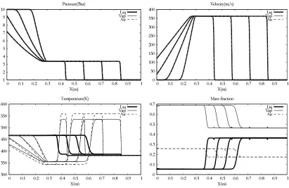
The Figure 1 shows the temporal evolution of some characteristic flow variables when the relaxation effects are absent. Only hydrodynamics solved by the Discrete Equations Method (DEM) is responsible for the evolution of all phases variables. As the volume fractions are initially uniform no interactions between phases are present. Then the results correspond to single-phase shock tube solutions and the evolution of the mass fractions comes from all the waves trajectories of each phase.
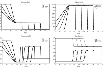
In the second case, the velocity and pressure relaxation effects are enabled. The associated results are presented in the Figure 2. No slip between phases is thus allowed. The mass fractions are then invariant across the shock wave and the rarefaction waves. As can be clearly seen in this figure all phases have the same pressure and the same velocity at each point and at each instant. But they have different temperatures. In this example, an interface problem is solved between two different mixtures. It clearly appears that interface conditions (equality of the pressure and the velocity) are fulfilled across interfaces.
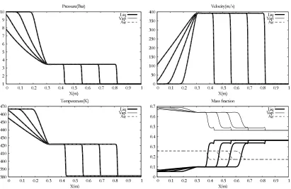
The instantaneous heat exchanges between phases are now taken into account. The corresponding results are presented in the Figure 3. All phases have a common temperature. In this figure we can notice that the shock wave velocity slightly decreased with respect to the preceding case. This is the direct consequence of the mixture sound speed decrease. Except the temperatures, few differences appear between this configuration and the last one.
!"!#
!$%&
'!!"!(
Figure 1. Numerical results of the three-phase shock tube without relaxation
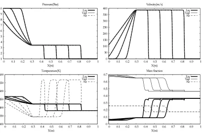
and vapor phases. The results are represented in the Figure 4. As can be clearly seen in the mass fraction graph evaporation and condensation occur across the shock wave and rarefaction waves respectively. The incondensable mass fraction obviously remains constant across the shock wave and the rarefaction waves. The common temperature now obeys the saturation temperature depending on the pressure. The shock wave velocity still decreased as well as the mixture sound speed.
In the last configuration heat exchanges between the incondensable and the liquid-vapor couple are disabled. The results are presented in the Figure 5. The thermal energy of the air is not accounted for the evaporation and condensation phenomena that are less important than the preceding case.
2.2.
Three-dimensional configuration
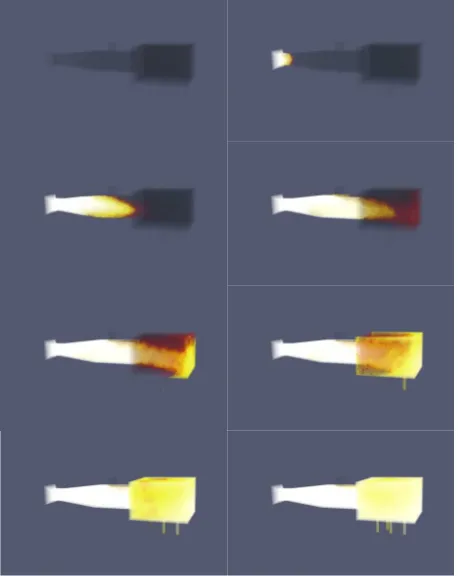
A three-dimensional configuration involving a cryogenic liquid flow is proposed in this section. Two inlets are considered in a pipe emerging in a confined tank containing 5 identical tubes as outlets. The boundary and initial conditions as well as the geometry are represented in the Figure 6. 50000 numerical cells (tetrahedrons) have been used to perform calculations.
Initially the whole domain is filled with helium. Cryogenic liquid and helium injections are also considered. The outlet pressure is uniform during the simulations. The vapor phase is initially present at a small quantity : αvap= 10−5.
First the heat exchanges between the 3 phases are enabled. The pressure and temperature relaxation procedure is then used.
) * + , . /
) * + , - . / 0 1 )
2345 67889:7;<=>?
@=A B7C D=: )
* + , -. / 0 1 )
) * + , - . / 0 1 )
2345 E:F88G:F3H7:5
@=A B7C D=:
-) )-* *-+ +-,
) * + , - . / 0 1 )
2345 BFI>;=<J34K85
@=A B7C D=:
+ +-, , - --.
) * + , - . / 0 1 )
2345 LF4CF:7<G:F3M5
@=A B7C D=:
Figure 2. Numerical results of the three-phase shock tube with pressure and velocity relax-ations : mixture at mechanical equilibrium
In this figure it can be seen that the cryogenic liquid jet which dynamics is slightly influenced by the helium injection gradually fills the system under consideration. The vapor phase still remains at small quantities during the simulation.
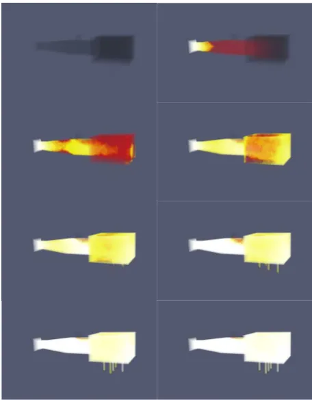
With the same configuration (6), evaporation and condensation are now allowed by using the Gibbs free energy relaxation procedure. The results corresponding to the temporal evolution of the mixture density are repre-sented in the Figure 8 at the same instants.
Since the liquid injection vapor appears at the divergent of the nozzle. The pressure drop and the strong differ-ence between the liquid and helium temperatures lead to an important liquid evaporation. The created vapor is ejected at high velocity (100m/sapproximately) towards the tank and the outlets. Then the thermodynamic equilibrium between the liquid and its vapor is subject to changes as the ambient pressure increases inside the medium : condensation takes place instead of evaporation at the end of the simulation. In this context a quasi-steady flow is obtained where the cryogenic liquid nearly fills the whole domain with helium.
Conclusion
The numerical results presented in this paper have shown the ability of the relaxation procedures to reproduce multiphase flows where instantaneous heat and mass transfer are involved. In fact these results correspond to limit flow configurations. As in [7] the associated limit models should be investigated and studied for each relaxation procedure.
N NO P NOQ NOR NOS NO T NO U NO V
N NOP NOQ NOR NOS NO T NO U NOV NOW NOX P YZ[\
]^__`a^bcdef
gdh i^j kda P
Q R S T U V W X PN
N NOP NOQ NOR NOS NO T NO U NOV NOW NOX P YZ[\
lam__namZo^a\
gdh i^j kda
p qp rpp rqp spp sqp tpp tqp upp
p pvr pvs pvt pvu pvq pvw pvx pvy pvz r {|}~
|}~
RUN RWN SN N SQN SSN SUN SWN
N NO P NOQ NOR N OS NO T NOU NOV NOW NOX P YZ[\
m[jma^cnamZ\
gdh i^j kda
Figure 3. Numerical results of the three-phase shock tube with velocity, pressure and tem-perature relaxations : mixture at mechanical and thermal equilibrium
of the flow topology appearing inside the multiphase medium. Nevertheless some additional efforts should be made to model the exchange area in simple configurations at least (bubbly flows with several particle sizes).
References
[1] Abgrall, R. &Saurel, R. (2003) Discrete equations for physical and numerical compressible multiphase mixtures.J. Comp. Physics,186, pp 361-396
[2] Baer, M.R. &Nunziato, J.W. (1986) A two-phase mixture theory for the deflagration-to-detonation transition (DDT) in reactive granular materials.Int. J. of Multiphase Flows,12, pp 861-889
[3] Barberon, T. &Helluy, P. (2005) Finite volume simulation of cavitating flows.Computers & Fluids,34, pp 832-858 [4] Berry, R.A.,Saurel, R. &Le M´etayer, O. (2010) The discrete equation methods (DEM) for fully compressible, two-phase
flows in ducts of spatially varying cross-section.Nuclear Engineering & Design,240, pp 3797-3818
[5] Chinnayya, A.,Daniel, E. &Saurel, R. (2004) Modelling detonation waves in heterogeneous energetic materials.J. Comp. Physics,196, pp 490-538
[6] Delhaye, J.M. (2001) Some issues related to the modeling of interfacial areas in gas-liquid flows I. The conceptual issues.C. R. Acad. Sci. Paris, S´erie IIb,329, pp 397-410
[7] Flatten, T.,Morin, A. &Munkejord, S.T. (2010) Wave propagation in multicomponent flow models.SIAM J. Appl. Math., 70, pp 2861-2882
[8] Harlow, F. &Amsden, A. (1971) Fluid dynamics.monograph LA-4700, Los Alamos National Laboratory, NM
[9] Helluy, P. &Seguin, N. (2006) Relaxation models of phase transition flows.Mathematical Modelling and Numerical Analysis, 40(2), pp 331-352
[10] Lallemand, M.-H.,Chinnayya, A. & Le M´etayer, O. (2005) Pressure relaxation procedures for multiphase compressible flows.Int. J. Num. Methods in Fluids,49, pp 1-56
[11] Layes, G. &Le M´etayer, O. (2007) Quantitative numerical and experimental studies of the shock accelerated heterogeneous bubbles motion.Physics Fluids,19, 042105
¡¢¢£¤¡¥¦§¨©
ª§« ¬¡ ®§¤ ¯
° ± ² ³ ´ µ ¶ · ¯¸
¸ ¸¹¯ ¸¹° ¸¹± ¸¹² ¸¹³ ¸¹´ ¸¹µ ¸¹¶ ¸¹· ¯ º»¼½
¾¿ÀÁÁ¿À»ÃÄ¿½
ÅÆÇ ÈÄÉ ÊÆ¿
¸ ³¸ ¯¸¸ ¯³¸ °¸¸ °³¸ ±¸¸ ±³¸ ²¸¸
¸ ¸¹¯ ¸¹° ¸¹± ¸¹² ¸¹³ ¸¹´ ¸¹µ ¸¹¶ ¸¹· ¯ º»¼½
ÈÀËÌÍÆÎÏ»¼ÐÁ½
ÅÆÇ ÈÄÉ ÊÆ¿
ÑÒÒ¤¡¦Ó¤ÒÔ
ª§« ¬¡ ®§¤
Figure 4. Numerical results of the three-phase shock tube with velocity, pressure, temperature and Gibbs free energy relaxations : mixture at total thermodynamic equilibrium
[13] Le M´etayer, O.,Massoni, J. &Saurel, R. (2005) Modelling evaporation fronts with reactive Riemann solvers.J. Comp. Physics,205(2), pp 567-610
[14] Lhuillier, D.,Morel, C. &Delhaye, J.M. (2000) Bilan d’aire interfaciale dans un m´elange diphasique : Approche locale vs approche particulaire.C. R. Acad. Sci. Paris, S´erie IIb,328, pp 143-149
[15] Saurel, R. &Abgrall, R. (1999) A multiphase Godunov method for compressible multifluid and multiphase flows.J. Comp. Physics,150, pp 425-467
[16] Saurel, R., Gavrilyuk, S. & Renaud, F. (2003) A Multiphase model with internal degrees of freedom : Application to shock-bubble interaction.J. Fluid. Mechanics,495, pp 283-321
[17] Saurel, R. &Le M´etayer, O. (2001) A multiphase model for compressible flows with interfaces, shocks, detonation waves and cavitation.J. Fluid. Mechanics,431, pp 239-271
[18] Saurel, R.,Massoni, J. &Renaud, F. (2007) A numerical method for one-dimensional compressible multiphase flows on moving meshes.Int. J. Num. Methods in Fluids,54(12), pp 1425-1450
Õ ÕÖ × ÕÖØ ÕÖÙ ÕÖÚ ÕÖ Û ÕÖ Ü ÕÖ Ý
Õ ÕÖ× ÕÖØ ÕÖÙ ÕÖÚ ÕÖ Û ÕÖ Ü ÕÖÝ ÕÖÞ ÕÖß × àáâã
äåææçèåéêëìí
îëï ðåñ òëè ó
ô õ ö ÷ ø ù ú û óü
ü üýó üýô üýõ üýö üý÷ üýø üýù üýú üýû ó þÿ
ÿ
ü ÷ü óüü ó÷ü ôüü ô÷ü õüü õ÷ü öüü
ü üýó üýô üýõ üýö üý÷ üýø üýù üýú üýû ó þÿ
!"ÿ#
ÙÕ Õ ÙÛÕ ÚÕ Õ ÚÛÕ ÛÕ Õ ÛÛÕ ÜÕ Õ
Õ ÕÖ × ÕÖØ ÕÖÙ Õ ÖÚ ÕÖ Û ÕÖÜ ÕÖÝ ÕÖÞ ÕÖß × àáâã
âñèåêèáã
îëï ðåñ òëè
Figure 5. Numerical results of the three-phase shock tube with velocity, pressure, temperature (liquid-vapor couple only) and Gibbs free energy relaxations : mixture at partial thermody-namic equilibrium
Helium
K T=280
Bar P=1
Outlets Helium injection
K T0=280
Cryogenic liquid injection
K T0=90
Bar P 1=