Efficiency of DMUs in Presence of New Inputs and Outputs in DEA

(1)

777

Available online at http://ijdea.srbiau.ac.ir

Int. J. Data Envelopment Analysis (ISSN 2345-458X)

Vol.3, No.3, Year 2015 Article ID IJDEA-00333, 9 pages

Research Article

Efficiency of DMUs in Presence of

New Inputs and Outputs in DEA

Esmat Noroozi

a*

, Elahe Sarfi

b

,

Farhad Hosseinzadeh Lotfi

c

(a) Department of Mathematics, East Tehran Branch, Islamic Azad University, Tehran, Iran (b) Department of Mathematics, Damghan Branch, Islamic Azad University, Damghan, Iran (c) Department of Mathematics, Science and Research Branch, Islamic Azad University, Tehran,

Iran

Received 2 January 2016, Revised 16 March 2016, Accepted 19 April 2016 Abstract

Examining the impacts of data modification is considered as sensitivity analysis. A lot of studies

have considered the data modification of inputs and outputs in DEA. The issues which has not heretofore been considered in DEA sensitivity analysis is modification in the number of inputs and

(or) outputs and determining the impacts of this modification in the status of efficiency of DMUs. This paper is going to present systems that show the impacts of adding one or multiple inputs or

outputs on the status of efficiency of DMUs and furthermore a model is presented for recognizing the minimum number of inputs and (or) outputs from among specified inputs and outputs which can be

added whereas an inefficient DMU will become efficient. Finally the presented systems and model have been utilized for a set of real data and the results have been reported.

Keywords

:

Data envelopment analysis; Sensitivity analysis; efficiency.

*

Corresponding Author: [email protected]

(2)

1. Introduction

Data envelopment analysis (DEA) is a

nonparametric approach for evaluating the relative efficiency of DMUs with multiple

inputs and multiple outputs. The basic models of DEA (Charnes et al, 1978; Banker et al,

1984 and Charnes et al ,1985) are used for evaluating of relative efficiency in similar economical systems. DEA has been extended

in different areas these days. For example

consider sensitivity analysis. Sensitivity analysis of DEA models which is based on the

linear programming are both theoretically and practically important. The first DEA sensitivity analysis paper by (Charnes et al

,1985) determined change in a single output. later many studies have been conducted in

changing some ofthe inputs and (or) outputs simultaneously by (Seiford et al ,1998; Zhu

,2001; Cooper et al, 2001;G.R.Jahanshahloo et

al,2004; Jahanshahloo et al,2005a;

Jahanshahloo et al,2005b) and etc.Heretofore one of the important issues which has considered in DEA sensitivity analysis is

modification (increasing or decreasing) in the value of the inputs and (or) out puts. In this

paper is going to investigate the impact of

increasing the number of the inputs and (or) out puts on the status of efficiency in DMUs.

The present study has been organized as follows: First some basic DEA models and related concepts have been reviewed.

Thereafter the number of inputs and (or) outputs has been modified and the impact of

this modification (adding of one or multiple inputs and outputs) has been presented through

some systems show the status of efficiency or inefficiency in DMUs and a model is

presented for recognizing the minimum number of inputs and (or) outputs from among

specified inputs and outputs which can be added whereas an inefficient DMU will

become efficient. Then a set of DMUs have been presented. By changing (adding) the number of inputs and (or) outputs, the

presented systems and a model in former

section have been utilized for this set of DMUs and the results have been reported. Finally the

results have been synthesized and conclude. 2. preliminary

Suppose n DMUs are evaluated, each of them

consumes m inputs to produce s outputs.

Suppose. Xj = x1j , x2j, … , xmj T and Yj =

(y_1j, y_2j, … , y_sj) T_{are as the inputs and outputs}

of DMUjfor j=1,…,n. For the first time (Charnes

et al, 1978) laid the foundation of DEA through introducing the CCR model. The multiplier form

of this model is as follows:

Max uryro s

r=1

S. t. vixio= 1 m

i=1

uryrj− vixij ≤ 0 m

i=1 s

r=1

j = 1, … , n (1)

ur≥0 r = 1, … , s

𝑣𝑖≥0 𝑖 = 1, … , 𝑚

That O is the index of the evaluated DMU and

U= (𝑢1, 𝑢2, … , 𝑢𝑠) є 𝑅𝑠and V= 𝑣1, 𝑣2, … , 𝑣𝑚 𝜖𝑅𝑚

Definition1. DMUois called CCR efficient if

(3)

E. Noroozi, et al /IJDEA Vol3, No.3, (2015). 777-785

779

1) sr=1ur∗yro = 1

2) At least in one optimal solution of this model u_r > 0 𝑓𝑜𝑟 𝑒𝑎𝑐ℎ 𝑟 = 1,2, … , s and v_i >

0 for each i=1,2,…,m.

If both conditions are acknowledged DMU_o is called strong efficient and if just first condition is acknowledged DMUo is called weak

efficient.

Definition2. DMU_o is called CCR inefficient if and only if s_r=1u_r∗y_ro < 1.

3. Adding of one or multiple inputs and (or)

outputs

Suppose 𝐷𝑀𝑈𝑜 with m inputs and s outputs

have been evaluated efficient. The optimal

value of objective function in model (1) will

not be worse through the addition of one or multiple inputs and (or) outputs because

adding input or output is equivalent to adding a new variable in model (1) ,so it is still preserved its efficiency. Then the inefficient

DMUs are considered. In this section some systems has been presented for adding of one

or multiple inputs and (or) outputs which by utilizing them it can be recognize the impact of

these modification. Furthermore a model is presented for recognizing the minimum

number of inputs and (or) outputs from among specified inputs and outputs which can be added whereas an inefficient DMU will

become efficient.

3.1 Adding of one input or output

Suppose 𝐷𝑀𝑈𝑜 is an inefficient DMU. Now

it’s going to present a system to find out

whether 𝐷𝑀𝑈𝑜 is preserved its inefficiency or

it has been changed to efficient with adding of one input ((m+1)th input). For this reason

consider the following system.

𝑢𝑟 𝑠

𝑟=1

𝑦𝑟𝑜= 1

𝑣𝑖 𝑚

𝑖=1

𝑥𝑖𝑜+ 𝑡𝑥 𝑚 +1 𝑜= 1

𝑢𝑟 𝑠

𝑟=1

𝑦𝑟𝑗− 𝑣𝑖 𝑚

𝑖=1

𝑥𝑖𝑗− 𝑡𝑥 𝑚+1 𝑗 ≤ 0

𝑢𝑟≥ 0 𝑗 = 1, … , 𝑛

𝑣𝑖≥ 0 𝑟 = 1, … , 𝑠

𝑡 ≥ 0 𝑖 = 1, … , 𝑚

(2)

In above system the new input 𝐷𝑀𝑈𝑗 for

𝑗 = 1, … , 𝑛 with 𝑥 𝑚 +1 𝑗 and its corresponding

weight is illustrated by t. The first constraint is the condition of efficiency for 𝐷𝑀𝑈_𝑜 and the other constraints are the constrains of model (1)

in presences of the new input.

Theorem 1. Suppose that 𝐷𝑀𝑈𝑜 has been

evaluated inefficient with m inputs and s outputs.

a) If system (2) is feasible then 𝑡 > 0 and with

adding input (m+1)th, 𝐷𝑀𝑈𝑜will become

efficient.

b) If system (2) is infeasible then with adding input (m+1)th, 𝐷𝑀𝑈_𝑜 will become inefficient. Proof a) Suppose that system (2) is feasible and t=0. Therefore model (1) has a feasible

solution with value of objective function equals one. This means 𝐷𝑀𝑈𝑜 has been

efficient in absence of the new input that is in

contradiction with inefficiency assumption of

𝐷𝑀𝑈𝑜. Now it should be proved that 𝐷𝑀𝑈𝑜

becomes efficient in presence of the new input. Consider the feasible solution of system (2)

(4)

with value of objective function equals one.

Max 𝑢𝑟𝑦𝑟𝑜 𝑠

𝑟=1

S. t. 𝑣𝑖𝑥𝑖𝑜+ 𝑡𝑥 𝑚+1 𝑜= 1 𝑚

𝑖=1

𝑢𝑟𝑦𝑟𝑗 − 𝑠

𝑟=1

𝑣𝑖𝑥𝑖𝑗− 𝑡𝑥 𝑚+1 𝑗 ≤ 0 𝑚

𝑖=1

𝑣𝑖≥ 0 𝑗 = 1, … , 𝑛 (3)

𝑢𝑟≥ 0 𝑖 = 1, … , 𝑚

𝑡 ≥ 0 𝑟 = 1, … , 𝑠

This means 𝐷𝑀𝑈𝑜 becomes efficient in

presence of the new input.

b) Suppose that system (2) is infeasible and

𝐷𝑀𝑈_𝑜 has become efficient in presence of the new input .Therefore in optimal solution of model (3), the value of objective function

equals one. This solution is feasible for system (2) that is in contradiction with the

infeasibility assumption of it. ∎

It is worthwhile note this point that if system (2) has alternative optimal solutions, decision

maker can choose any one of these solutions. System (2) can be generalized for adding on

output as follows:

𝑢𝑟 𝑠

𝑟=1

𝑦𝑟𝑜+ 𝑤𝑦 𝑠+1 𝑜= 1

𝑣𝑖 𝑚

𝑖=1

𝑥𝑖𝑜 = 1

𝑢𝑟 𝑠

𝑟=1

𝑦𝑟𝑗 − 𝑣𝑖 𝑚

𝑖=1

𝑥𝑖𝑗+ 𝑤𝑦(𝑠+1)𝑗 ≤ 0

𝑢𝑟≥ 0 𝑗 = 1, … , 𝑛

𝑣𝑖≥ 0 𝑟 = 1, … , 𝑠

𝑤 ≥ 0 𝑖 = 1, … , 𝑚 (4)

3. 2 Adding of multiple inputs and (or)

outputs

Now the impact of adding multiple inputs and

(or) outputs on inefficient 𝐷𝑀𝑈𝑜 is

considered. Suppose inputs (m+1),…,(m+k) and outputs (s+1),…,(s+h) are added to find

out whether 𝐷𝑀𝑈𝑜 is still preserved its

inefficiency or it will become efficient.

The following system is presented through the generalization of system (2) and (4):

𝑢𝑟𝑦𝑟𝑜+ 𝑤𝑞 ℎ

𝑞=1

𝑦 𝑠+𝑞 𝑜= 1 𝑠

𝑟=1

5

𝑢𝑟𝑦𝑟𝑗+ 𝑠

𝑟=1

𝑤𝑞𝑦 𝑠+𝑞 𝑗− 𝑣𝑖𝑥𝑖𝑗− 𝑡𝑝𝑥 𝑚 +𝑝 𝑗 ≤ 0 𝑘 𝑝=1 𝑚 𝑖=1 ℎ 𝑞=1

𝑗 = 1, … , 𝑛

𝑣𝑖𝑥𝑖𝑜+ 𝑡𝑝𝑥 𝑚 +𝑝 𝑜= 1 𝑘

𝑝=1 𝑚

𝑖=1

𝑣𝑖≥ 0 𝑖 = 1, … , 𝑚

𝑢𝑟≥ 0 𝑟 = 1, … , 𝑠

𝑡𝑝 ≥ 0 𝑝 = 1, … , 𝑘

𝑤𝑞≥ 0 𝑞 = 1, … , ℎ

]

Where 𝑥 𝑚 +𝑝 𝑗 and 𝑦 s+q j are respectively the

𝑝(th) input and 𝑞(th) output of 𝐷𝑀𝑈_𝑗 for

𝑝 = 1 … 𝑘 and 𝑞 = 1 … ℎ. Furthermore 𝑡𝑝 and

𝑤_𝑞 are respectively related weights to 𝑝(th) input and 𝑞(th) output.

Theorem 2. Suppose that 𝐷𝑀𝑈𝑜 has been

evaluated inefficient with m inputs and s

outputs.

a) If system (5) is feasible then at least one

element of 𝑡1, … , 𝑡𝑘, 𝑤1, … , 𝑤ℎ is positive.

Furthermore by adding these k inputs and h outputs 𝐷𝑀𝑈𝑜 will become efficient.

b) If system (5) is infeasible then by adding these 𝑘 inputs and ℎ outputs, 𝐷𝑀𝑈_𝑜 will still preserve its inefficiency.

Proof is similar to theorem 1.∎

4. Finding out the minimum number of

(5)

781

Suppose that inefficient 𝐷𝑀𝑈𝑜 has become

efficient by adding all of these 𝑘 inputs and ℎ

outputs. However it may be not necessary to add all these inputs and outputs for becoming

𝐷𝑀𝑈𝑜 efficient. Now the question that will be

raised is finding the minimum number of inputs and (or) outputs from among k inputs

and h outputs which can be added whereas inefficient 𝐷𝑀𝑈𝑜 becomes efficient. For this

reason the following model can be presented.

𝑧∗_{= 𝑀𝑖𝑛 𝑑}

𝑝+ 𝑑𝑞′ ℎ

𝑟=1 𝑘

𝑝=1

S. t. 𝑢𝑟𝑦𝑟𝑜+ 𝑤𝑞 ℎ

𝑞=1

𝑦 𝑠+𝑞 𝑜= 1 𝑠

𝑟=1

𝑟 =1

𝑤𝑞𝑦 𝑠+𝑞 𝑗 ℎ

𝑞=1

− 𝑣𝑖𝑥𝑖𝑗− 𝑡𝑝𝑥 𝑚+𝑝 𝑗≤ 0 𝑘

𝑝=1 𝑚

𝑖 =1

𝑗 = 1, … , 𝑛 (6)

𝑣𝑖𝑥𝑖𝑜+ 𝑡𝑝𝑥(𝑚 +𝑝)𝑜= 1 𝑘

𝑝=1 𝑚

𝑖=1

0 ≤ 𝑡𝑝 ≤ 𝑀𝑑𝑝 𝑝 = 1, … , 𝑘

0 ≤ 𝑤𝑞≤ 𝑀𝑑𝑞′ 𝑞 = 1, … , ℎ

𝑑𝑝∈ 0,1 𝑝 = 1, … , 𝑘

𝑑𝑞′ ∈ 0,1 𝑞 = 1, … , ℎ

𝑣𝑖≥ 0 𝑖 = 1, … , 𝑚

𝑢𝑟≥ 0 𝑟 = 1, … , 𝑠

𝑡𝑝 ≥ 0 𝑝 = 1, … , 𝑘

𝑤𝑞≥ 0 𝑞 = 1, … , ℎ

Theorem 3. If 𝐷𝑀𝑈𝑜 becomes efficient with

adding all of these 𝑝 inputs and ℎ outputs then

Model (6) is feasible.

Proof Since 𝐷𝑀𝑈𝑜 has become efficient then

the following model has a feasible solution

with value of objective function equals one.

𝑧∗_{= 𝑀𝑖𝑛 𝑢}

𝑟𝑦𝑟𝑜+ 𝑤𝑞 ℎ

𝑞=1

𝑦 𝑠+𝑞 𝑜

𝑠

𝑟=1

S. t. 𝑣𝑖𝑥𝑖𝑜+ 𝑡𝑝𝑥 𝑚 +𝑝 𝑜= 1 𝑘

𝑝=1 𝑚

𝑖=1

𝑟=1

𝑤𝑞𝑦 𝑠+𝑞 𝑗 ℎ

𝑞=1

− 𝑣𝑖𝑥𝑖𝑗− 𝑡𝑝𝑥(𝑚+𝑝)𝑗≤ 0 𝑘

𝑝=1

𝑚

𝑖=1

𝑗 = 1, … , 𝑛 (7)

𝑣𝑖≥ 0 𝑖 = 1, … , 𝑚

𝑢𝑟≥ 0 𝑟 = 1, … , 𝑠

𝑡𝑝 ≥ 0 𝑝 = 1, … , 𝑘

𝑤𝑞≥ 0 𝑞 = 1, … , ℎ

The optimal solution of the above model with

𝑑𝑝 = 1 for 𝑝 = 1, … , 𝑘 and 𝑑𝑞′ = 1 for 𝑞 =

1, … , ℎ is a feasible solution for model (6). ∎

Theorem 4 . The minimum number of inputs and (or) outputs among these 𝑘 inputs and ℎ

outputs which should be added whereas inefficient 𝐷𝑀𝑈𝑜 will become efficient, equals

𝑧∗_.

Proof With regard to minimization of model (6) it’s evident that the binary variables 𝑑_𝑝∗ _and_𝑑′

𝑞 ∗

for 𝑝 = 1, … , 𝑘 and 𝑞 = 1, … , ℎ are preferred to

choose zero value. So by regarding to the

constraints 0 ≤ 𝑡𝑝 ≤ 𝑀𝑑𝑝 and 0 ≤ 𝑤𝑞 ≤

𝑀𝑑_𝑞′_{, if}_𝑑

𝑝∗ = 0 (𝑑′𝑞∗ = 0) then 𝑡𝑝∗ = 0 (𝑤𝑞∗ =

0). It means 𝑚 + 𝑝 th input( 𝑠 + 𝑞 th output)

cannot be added. On the other hand if 𝑑𝑝∗ = 1

(𝑑′𝑞∗ = 1) then 𝑡𝑝∗ > 0(𝑤𝑞∗> 0). It means the

corresponding input (output) should be added.

So 𝑘𝑝=1𝑑𝑝+ ℎ𝑟=1𝑑𝑞′ indicates the number of

added inputs and or outputs. With regard to this issue and feasibility of model (6), it can be concluded that 𝑧∗ equals the minimum number of inputs and (or) outputs among these 𝑘 inputs

(6)

that the inefficient 𝐷𝑀𝑈𝑜 will become

efficient.∎

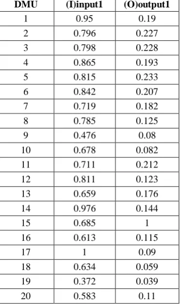
5. Empirical example

Now the presented systems and model in this

paper are used for the data of tables 1and 2 related to twenty DMUs with three inputs and

three outputs. These data are real and extracted from (Alder et al, 2002).The original data and

the data that are supposed to be add are given respectively in table 1 and table 2. Evaluating

the presented DMUs in table 1 through CCR model has been revealed that only 𝐷𝑀𝑈15 is

efficient.

Table 1. Data of input1 and output1of DMUs (Alder et al , 2002)

Table2. Data of input2,3 and output2,3 of DMUs (Alder et al, 2002)

DMU (I) input2

(I) input3

(O) output

2

(O) output

3

1 0.7 0.155 0.521 0.293

2 0.6 1 0.627 0.462

3 0.75 0.513 0.97 0.261

4 0.55 0.21 0.632 1

5 0.85 0.268 0.722 0.246

6 0.65 0.5 0.603 0.569

7 0.6 0.35 0.9 0.716

8 0.75 0.12 0.234 0.298

9 0.6 0.135 0.364 0.244

10 0.55 0.51 0.184 0.049

11 1 0.305 0.318 0.403

12 0.65 0.255 0.923 0.628 13 0.85 0.34 0.645 0.261

14 0.8 0.54 0.514 0.243

15 0.95 0.45 0.262 0.098 16 0.9 0.525 0.402 0.464

17 0.6 0.205 1 0.161

18 0.65 0.235 0.349 0.068

19 0.7 0.238 0.19 0.111

20 0.55 0.5 0.615 0.764

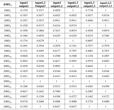
Now it’s going to present the results of adding

the inputs and outputs in table 2 on the status

of efficiency of DMUs in table 3. The results of table 3 are obtained through using the

software DEA-Solver.

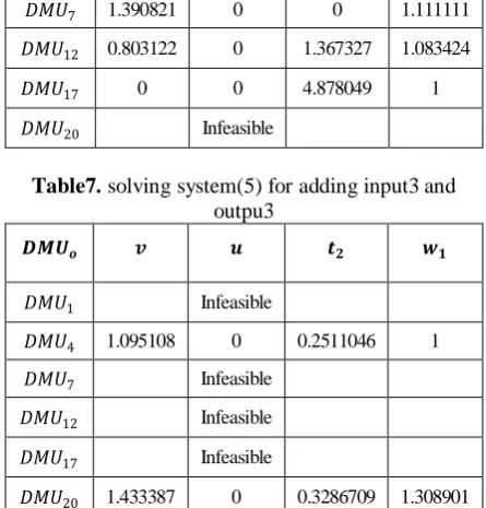
Now systems (2), (4) and (5) for adding one or

multiple inputs and or outputs are solved by using the software lingo. The related results for 𝐷𝑀𝑈_𝑜 = 𝐷𝑀𝑈₁, 𝐷𝑀𝑈₄, 𝐷𝑀𝑈₇, 𝐷𝑀𝑈₁₂,

, 𝐷𝑀𝑈₁₇𝑎𝑛𝑑 𝐷𝑀𝑈₂₀ are presented in tables 4, 5, 6, 7 and 8.

DMU (I)input1 (O)output1

1 0.95 0.19

2 0.796 0.227

3 0.798 0.228

4 0.865 0.193

5 0.815 0.233

6 0.842 0.207

7 0.719 0.182

8 0.785 0.125

9 0.476 0.08

10 0.678 0.082

11 0.711 0.212

12 0.811 0.123

13 0.659 0.176

14 0.976 0.144

15 0.685 1

16 0.613 0.115

17 1 0.09

18 0.634 0.059

19 0.372 0.039

(7)

783 Table 4.solving system (4) for adding output2

𝑫𝑴𝑼𝒐 𝒗 𝒖 𝒘𝟏

𝐷𝑀𝑈1 Infeasible

𝐷𝑀𝑈7 1.390821 0 1.111111

Table 5.solving system (4) for adding output3

𝑫𝑴𝑼𝒐 𝒗 𝒖 𝒘𝟏

𝐷𝑀𝑈20 1.715266 0 1.308901

𝑫𝑴𝑼𝒐 _output1input1 input1,2 _Output3 _output1,2 input1 _output1,2input1,3 _output1,3input1,3 _output1,2,3input1,2,3

𝐷𝑀𝑈1 0.1370 0.3317 0.4829 1 0.7738 1

𝐷𝑀𝑈2 0.1953 0.5677 0.6925 0.6925 0.5677 0.8334

𝐷𝑀𝑈3 0.1957 0.3973 0.9911 0.9911 0.4046 0.9911

𝐷𝑀𝑈4 0.1528 0.9173 0.6216 0.8719 1 1

𝐷𝑀𝑈5 0.1958 0.3804 0.7613 0.8974 0.4958 0.8974

𝐷𝑀𝑈6 0.1684 0.6076 0.6229 0.6229 0.6274 0.7484

𝐷𝑀𝑈7 0.1734 0.8278 1 1 0.8697 1

𝐷𝑀𝑈8 0.1091 0.3544 0.2878 0.7161 0.7677 0.7979

𝐷𝑀𝑈9 0.1151 0.4495 0.6177 0.7597 0.4863 0.7875

𝐷𝑀𝑈10 0.0828 0.1236 0.2500 0.2500 0.1236 0.2897

𝐷𝑀𝑈11 0.2042 0.5666 0.4617 0.5055 0.5974 0.6045

𝐷𝑀𝑈12 0.1039 0.6158 0.9092 1 0.6642 1

𝐷𝑀𝑈13 0.1829 0.4322 0.8166 0.8166 0.4492 0.8166

𝐷𝑀𝑈14 0.1011 0.2591 0.4413 0.4413 0.2681 0.4693

𝐷𝑀𝑈15 1 1 1 1 1 1

𝐷𝑀𝑈16 0.1286 0.6263 0.5515 0.5515 0.6263 0.6390

𝐷𝑀𝑈17 0.0617 0.1642 0.7989 1 0.2907 1

𝐷𝑀𝑈18 0.0637 0.1299 0.4398 0.4727 0.1462 0.4727

𝐷𝑀𝑈19 0.0718 0.2660 0.4088 0.4088 0.2729 0.4088

(8)

Table 6. solving system(5) for adding input3 and output2

𝑫𝑴𝑼𝒐 𝒗 𝒖 𝒕𝟐 𝒘𝟏

𝐷𝑀𝑈1 0.149183 2.311984 5.5372650 1.076244

𝐷𝑀𝑈7 1.390821 0 0 1.111111

𝐷𝑀𝑈12 0.803122 0 1.367327 1.083424

𝐷𝑀𝑈17 0 0 4.878049 1

Table7. solving system(5) for adding input3 and outpu3

𝑫𝑴𝑼𝒐 𝒗 𝒖 𝒕𝟐 𝒘𝟏

𝐷𝑀𝑈4 1.095108 0 0.2511046 1

𝐷𝑀𝑈20 1.433387 0 0.3286709 1.308901

Now by using model (6) is determined the

minimum number of inputs and or outputs that should be added in a way that the inefficient

units become efficient. For this purpose model (6) is solved through using the software Lingo

and the related results are presented in table 9 In table 9, 𝑧∗= 1 for 𝐷𝑀𝑈𝑜 = 𝐷𝑀𝑈7 and

𝐷𝑀𝑈₂₀ . This means the minimum number of

inputs and outputs among

input2, input3, output2, output3 that

should be added in a way that 𝐷𝑀𝑈7 and

𝐷𝑀𝑈₂₀ become efficient equals 1. The added inputs and (or) outputs for 𝐷𝑀𝑈7 and 𝐷𝑀𝑈20

are respectively outpt2 and output3. But

𝑧∗_{= 2}_for _𝐷𝑀𝑈

𝑜 = 𝐷𝑀𝑈1, 𝐷𝑀𝑈4, 𝐷𝑀𝑈12

and 𝐷𝑀𝑈₁₇. The added inputs and (or) outputs for 𝐷𝑀𝑈₁, 𝐷𝑀𝑈₁₂ and 𝐷𝑀𝑈₁₇ are input3 and output2 whereas the added inputs and (or)

outputs for 𝐷𝑀𝑈4 are input3 and output3.

(9)

785 6. Conclusion

In this paper is presented a system for showing

that whether inefficient 𝐷𝑀𝑈𝑜 is still

preserved its inefficiency or it will become efficient through adding a given input or

output. Next this system has been generalized for adding given multiple inputs and (or)

outputs. Afterwards a model is presented that can be obtained the minimum number of

inputs and outputs among the given inputs and outputs which should be added whereas

inefficient 𝐷𝑀𝑈𝑜will become efficient. Finally

the mentioned systems and model have been utilized in a set of DMUs and the results have

been presented.

References

[1] Alder, N., Fridman, L., & Sinuany-Stern,

Z. (2002). Review of ranking methods in

thedata envelopment analysis context. European Journal of Operational

Research,140, 249–265.

[2] Banker R D, Charnes A and Cooper W W. (1984). Some model for estimating technical

and scale inefficiencies in data envelopment analysis, Manage. Sci. 30: 1078-1092.

[3] Charnes A, Cooper W W, Rhodes E. (1978).Measuring the efficiency of decision

making units. European Journal of

Operational Research 2 (6): 429–444.

[4] Charnes A, Cooper W W, Lewin A Y,

Morey R C and Rousseau J J.

(1985).Sensitivity and stability analysis in

DEA. Annals of Operations Research 2: 139–

156.

[5] Cooper W W, Li S, Seiford L M, Tone K,

Thrall R M, Zhu J .(2001). Sensitivity and Stability Analysis in DEA: Some Recent

Developments, Journal of Productivity Analysis 15: 217-246.

[6] Jahanshahloo G R, HosseinzadehLotfi F and Moradi M .(2004).Sensitivity and Stability

analysis in DEA with interval data. Applied Mathematics and Computation 156:463-477.

[7] Jahanshahloo G R, Hosseinzadeh F, Shoja N, Sanei M and Tohidi G. (2005a).Sensitivity

and stability analysis in DEA. Applied Mathematics and Computation 169: 897-904. [8] Jahanshahloo G R, HosseinzadehLotfi F,

Shoja N, Tohidi G and Razavyan S. (2005b).A one-model approach to classification and

sensitivity analysis in DEA.Applied

Mathematics and Computation 169: 887-896.

[9] Seiford L M, Zhu J. (1998).Stability regions for maintaining efficiency in data

envelopment analysis. European Journal of Operations research 108: 127-139.

[10] Zhu J. (2001).Super-efficiency and DEA

sensitivity analysis. European Journal of