Model identification and dynamic analysis of ship propulsion shaft lines

Journal of Theoretical and Applied Vibration and Acoustics 1(2) 85-95 (2015)

* Corresponding Author: Hassan Jalali, Email: [email protected] I S A V

Journal of Theoretical and Applied

Vibration and Acoustics

journal homepage: http://tava.isav.ir

Model identification and dynamic analysis of ship propulsion

shaft lines

Hassan Jalali

a*

, Hamid Ahmadian

b

a

Department of Mechanical Engineering, Arak University of Technology, University St., Arak, Iran

b

Center of Excellence in Experimental Solid Mechanics and Dynamics, Iran University of Science and Technology, Narmak, Tehran, Iran

K E Y W O R D S A B S T R A C T

FE modeling Shaft line

Vibration measurement Updating

Campbell diagram

Dynamic response analysis of mechanical structures is usually performed by adopting numerical/analytical models. Finite element (FE) modeling as a numerical approach plays an important role in dynamic response analysis of complex structures. The calculated dynamic responses from FE analysis are only reliable if accurate FE models are used. There are many elements in real mechanical structures which make constructing accurate FE models difficult. For example, modeling the boundary supports of mechanical structures are usually challenging because of the uncertainties existing in their stiffness values. The stiffness values of boundary supports can be identified by using experimental natural frequencies and hence the FE model can be corrected. In this paper, the FE modeling and updating of propulsion shaft lines in a ship structure is considered by employing experimental modal parameters, i.e. natural frequencies. Natural frequencies of shaft lines are measured by performing experimental vibration testing. The corrected FE models are used and dynamic response analysis of shaft lines is conducted.

©2015 Iranian Society of Acoustics and Vibration, All rights reserved

1. Introduction

The propulsion system of a ship- consisting of main engine, gearbox, propulsion shaft line, propeller and pertinent auxiliary system- is used to propel the ship and to control its maneuvering. The essential part of a ship propulsion system is propulsion shaft line. The excitation forces originated from the shaft line can greatly affect the dynamic response of the whole ship structure. A reliable FE model of the shaft line is an assist in dynamic response prediction of the ship structure.

86 The power transmission system was modeled as a four degree-of-freedom system by Rao [5] using spring and damping elements. Damping elements were used between the main engine and the gearbox to reduce torsional vibrations, and between the thrust bearing and the propeller to reduce lateral vibrations. Connection of the main engine, gearbox, bearings and propeller to the foundation was modeled by using spring elements. Hara et al. [6] analyzed the torsional, axial and lateral vibrations of a main engine propeller shaft system with building block approach. The crankshaft was modeled by three dimensional solid elements. The propeller was considered as a material point and the added mass of water was taken into account by its mass, moment of inertia and polar moment of inertia. Equivalent spring elements were used to consider the bearing and foundation flexibilities.

FE model updating of rotor shafts has a long history in structural dynamics. Feng et al. [7] considered FE model updating of two rotor shafts by using several optimization techniques. They corrected the FE model of a general shaft and a shrinkage fitted shaft assembled with a disk by employing a genetic algorithm. Kwon and Lin [8] developed a method for selection of the frequency points in FRF-based model updating approach. They applied their method in the updating procedure of a rotor-bearing system. Tiwari et al. [9] reviewed the identification methods of dynamic parameters for bearings.

In this paper, dynamic analysis of a ship propulsion shaft lines is considered. For this end the shaft lines are modeled by using the finite element method. Experimental vibration testing is conducted on the shaft lines and their dynamic properties are measured. The flexibilities of the connection points in the shaft lines need to be considered precisely in order to obtain reliable FE models. Therefore the FE model of the shaft lines are corrected by using measured natural frequencies. Finally, the obtained accurate FE models are employed and the dynamic behavior of the shaft lines at different rotational speeds are investigated in terms of Campbell diagrams.

2. Problem statement

The propulsion system of a ship structure which consists of several elements is used to transmit thrust energy from the engine to the propeller. Different components of a ship propulsion system include: main engine, couplings, gearbox, bearings, shaft line, brackets and propeller. Two types of shaft lines- namely outer and inner shaft lines- are used in the propulsion system of the ship under consideration in this paper. The inner shaft line is monolithic but the outer shaft line is composed of three parts which are connected through rigid couplings. Also, the outer shaft line is longer than the inner shaft line which makes it more flexible. The extra flexibility of the outer shaft line reduces its natural frequency compared to the inner shaft line. The shaft lines are depicted in Fig. (1) and (2).

87 structure. The dynamic response of the shaft line can be investigated by using an accurate dynamic model. In the following section, dynamic modeling of the shaft lines is explained.

3. Theory

3.1. Dynamic modeling

The equation governing the dynamic response of a rotating shaft in a stationary reference frame is written as,

)} ( { )} ( ]{ [ )} ( ]){ [ ] ([ )} ( ]{

[M qt  C G q t  K q t  f t (1)

where

_{ }

M ,

_{ }

C ,

_{ }

G and

_{ }

K are the mass, damping, gyroscopic and stiffness matrices

respectively.

_

q t( )

_

and

_

f t( )

_

are the system response and external forcing vectors and  is the shaft rotational speed. The free vibration of an un-damped rotating shaft is governed by,

} 0 { )} ( ]{ [ )} ( ]{ [ )} ( ]{

[M qt G q t  K q t  (2)

The Campbell diagram which is the curve of natural frequencies versus rotating speed can be used to obtain the critical speeds. In fact the intersection points of natural frequency lines and excitation frequency lines are the critical speeds. The critical speeds can also be obtained by solving a new eigen problem as described in the following.

The synchronous motion of a rotating shaft (i.e. Eq. (2)) occurs when the response of Eq. (2) is considered in the following form,

t j e t

q()} {} 

{  (3)

where  and {} are respectively the natural frequency and the mode shape. By substituting Eq. (3) into Eq. (2) and knowing that at critical speeds  , Eq. (4) is obtained,

0 } ]){ [ ]

([K 2 M   (4)

where _M _

 

M  j G

 

. The critical speeds of the rotating shaft are the natural frequencies obtained from Eq. (4).

3.2. Model correction

There are usually parts in real structures- for example joints or connections- which their modeling or model parameters are uncertain when constructing FE models. The FE models can be updated and the unknown joints or connection parameters can be identified by using experimental results and employing the eigen-sensitivity approach. In the eigen-sensitivity approach, variation in the jth natural frequency is related to the change in design parameters

N i

88 n j p p N i i i j

j , 1,2,...,

1 2 2      

_

   (5) 2 j i p  

 is the sensitivity of

th

j natural frequency with respect to p_i and can be calculated as described in the following. The FE model is corrected by using the natural frequencies measured when  0. From Eq. (4) and by setting  0 one obtains,

0 } ]){ [ ]

([K 2_j M _j  (6)

In Eq. (6) _j is the natural frequency. By taking differentiation of Eq. (6) with respect to

parameter p_i the following equation is obtained,

0 } ){ ] [ ] [ ] [ ( 2 2          j i j i j i p M M p p K    (7)

Pre-multiplying Eq. (7) with

 

j T, assuming that the mode shapes are mass normalized i.e.

 

_j T

 

M

 

_j 1and after some algebraic manipulations one can conclude that,

} { ] [ } { } { ] [ } { 2 2 j i T j j j i T j i j p M p K

p     

         (8)

By substituting Eq. (8) into Eq. (5) and writing Eq. (5) for n natural frequencies, the FE model updating problem is formulated as,

                                                           n n N T n na n N T n n T n na n T n N T a N T T a T na ne a e p p p M p K p M p K p M p K p M p K        1 2 1 2 1 1 1 2 1 1 1 1 1 1 2 1 1 1 1 2 2 2 1 2 1 } { ] [ } { } { ] [ } { } { ] [ } { } { ] [ } { } { ] [ } { } { ] [ } { } { ] [ } { } { ] [ } {                         (9)

where _ne and _na are the natural frequencies from experiment and FE analysis respectively. By considering some initial values for the parameters p_i, Eq. (9) is solved iteratively and the initial values are updated. Updated parameters in the rth iteration is obtained as r r 1 r

i i i

p p  p

   . Parameter correction is continued until the norm of differences between experimental and FE models become less than some pre-determined values, i.e.

   

2 2

e a

   . In the following section, FE modeling of the shaft lines is described.

4. FE modeling

89 lengths of inner and outer shaft lines are respectively 10.8 m and 17.0 m. The shaft lines have a solid cross section with an outer diameter of 0.14 m in most of their parts. The inner shaft line was mounted on the ship by using two brackets and one bearing. The outer shaft line was mounted by using three brackets and two bearings. There were also two supports for each shaft line in the gearbox. The Solid45 element of Ansys software is used in FE modeling of the shaft lines. Since the engine and the gearbox are connected by using a flexible coupling, the dynamics of the engine does not affect the dynamics of the rest of the propulsion system. Therefore in FE modeling of the shaft lines, the engine is not modeled. The effects of the shaft lines’ supports are considered by using linear springs. Therefore, the brackets, the internal bearing, the astern tube and the bearings of the gearbox are modeled by using spring elements in the lateral and vertical directions. The FE models of the shaft lines are presented in Fig. (1) and (2).

Fig. 1. FE model of the inner shaft line

The shaft lines are made of steel and the material properties of E=210 Gpa, =7800 kg/m3 and

=0.3 are used in FE modeling.

Fig. 2. FE model of the outer shaft line

In the FE models shown in Fig. (1) and (2), the propeller is represented by a solid disk with mass and inertial properties equal to the real propeller. It is worth mentioning that the propeller and a section of the shaft lines- i.e. the section between the astern tube and propeller- are in water. Therefore, the mass effects of water are added to the FE models of these sections. For example the added mass moment of inertia to the propeller caused by water is calculated by using Eq. (10) (MacPherson et.al [10]),

z

EAR D C

D C

IE IE w IE

  

2 2 5 0.0703( / )

, 

90 where _w is the water mass density, D is the propeller diameter, EAR is the propeller expanded area ratio and z is the number of propeller blades. The stiffness coefficients of the support springs in the FE models shown in Fig. (1) and (2) are unknown. These coefficients can be identified by updating the FE models using the experimental natural frequencies of the shaft lines. In the next section, the experimental vibration testing conducted on the shaft lines is explained.

5. Experimental vibration testing

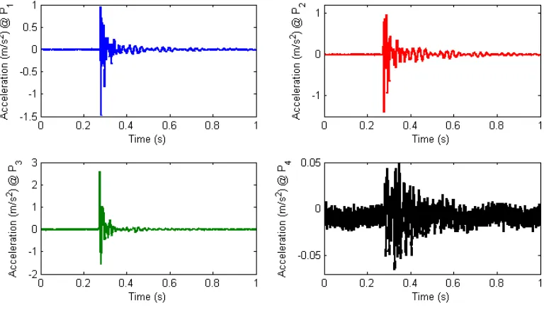
Experimental vibration testing is performed on the shaft lines at zero rotational speed, i.e.  0, in order to record their dynamic responses; the recorded dynamic responses are used later in this section and the natural frequencies of the shaft lines are extracted. The shafts were tested at their actual use condition, i.e. when they were mounted on the ship. It is well known from classic vibration theory that only the natural modes contribute in constructing the free vibration response of structures. Therefore, the natural frequencies can be obtained by analyzing the measured free responses of the shaft lines. In order to measure the free responses, the shaft lines are excited by using hammer and their dynamic response is measured by employing DJB A/120/V accelerometers. Four measurement points- three on the outer shaft line and one on the inner shaft line- are selected for performing the vibration tests. The shaft lines are excited at each point individually by hammer and the response of all measurement points are recorded. A NI USB-4431 data acquisition module is used for digitizing the acceleration response signals. The digitized signals are then recorded for future analysis. A schematic of the measurement setup is presented in Fig. (3).

Fig. 3. Schematic of the measurement set-up

In Fig. (4) the hammer used for exciting the shaft lines and one of the accelerometers used for measuring the shaft line free vibration response are shown. A measured dynamic response due to exciting point P1 is presented in Fig. (4). Due to the presence of damping in the shaft lines, the

91 frequency contents of the recorded response signals represent the natural frequencies of the shaft lines.

Fig. 4. Exciting a shaft line by hammer (left) and measuring its dynamic response (right)

Fig. 5. Measured acceleration signals

The frequency contents of the signals can be extracted by transferring the signals from time to frequency domain. The Continuous Wavelet Transform (CWT) is employed to decompose the recorded signals and hence to obtain the natural frequencies (Chen et.al. [11]). The CWT for a time domain signal is defined as,





 

 

   

 W a b a x a b g d

x( )} x( , ) ( ) ( )

{ *

92 where a and b are dilation and translation parameters and g is the Morlet wavelet function which is defined as Eq. (12). It is worth mentioning that in Eq. (11), *

( )

g  denotes the complex conjugate,

2 0 ( 1/2) )

( _ej _e t g _  

 (12)

where ₀ is a tunable parameter. W a bx( , ) is a complex function and it can be shown that if ( )x is the free vibration response of a structure, the following equations can be used to obtain the natural frequencies and damping ratios,

1 0, )

(

lnW_x a b _nbc (13)

2 0, )

(a b b c W_x  _d 

  (14)

in Eq.s (13) and (14), a₀ is the point at which W a b_x( , ) is maximum,  is the damping ratio,

n

 is the natural frequency and _d is the damped natural frequency, i.e. 2

1

d n

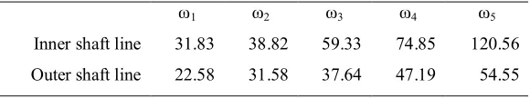
   . By using the theory explained above, the natural frequencies of the shaft lines are obtained. Table (1) shows the first five natural frequencies of the shaft lines,

Table 1. The experimental natural frequencies (Hz) ω5

ω4

ω3

ω2

ω1

120.56 74.85

59.33 38.82

31.83 Inner shaft line

54.55 47.19

37.64 31.58

22.58 Outer shaft line

The natural frequencies presented in Table (1) are used in the next section and the FE models are corrected.

6. FE model correction

As it was stated in the preceding sections, the stiffness values of the supports used in the FE models of the shaft lines, i.e. k_i, k_i, i1, 2,...,5 are uncertain. A set of reliable vales for support stiffness coefficients can be obtained by updating and correcting the FE models. FE model correction is done by minimizing the norm of differences between experimental natural frequencies and the natural frequencies obtained from FE model. The objective function in this minimization problem is defined as (Mottershead and Friswell [12]),

} { } { } { } { min

: fem

T fem ex

T ex

OBJ      (15)

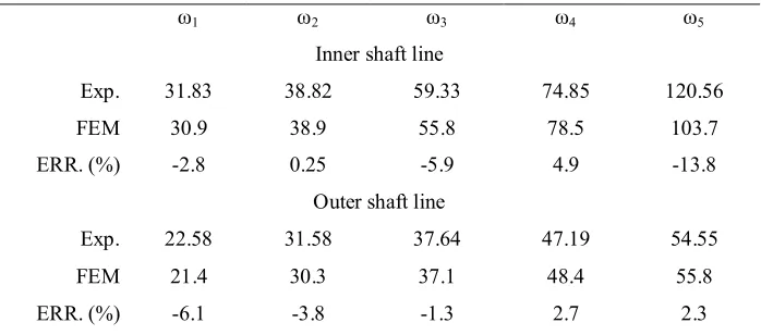
93 then identified by minimizing the objective function of Eq. (15). The identified stiffness parameters for the inner and outer shaft lines are presented in Table (2),

Table 2. The identified support stiffness parameters (MN/m)

1

k k₂ k₃ k4 k5

72.7 193 227 107.7 86.7

1

k k₂ k3 k4 k5

73.2 243.7 131 160.5 172

In order to measure the accuracy of the updated FE models, the experimental natural frequencies are compared with the natural frequencies obtained from updated FE models in Table (3),

Table 3. Experimental and updated natural frequencies (Hz) ω5

ω4

ω3

ω2

ω1

Inner shaft line

120.56 74.85

59.33 38.82

31.83 Exp.

103.7 78.5

55.8 38.9

30.9 FEM

-13.8 4.9

-5.9 0.25

-2.8 ERR. (%)

Outer shaft line

54.55 47.19

37.64 31.58

22.58 Exp.

55.8 48.4

37.1 30.3

21.4 FEM

2.3 2.7

-1.3 -3.8

-6.1 ERR. (%)

Results presented in Table (3) show that the updated FE models are well capable to regenerate the natural frequencies of the real shaft lines. This indicates that the FE models constructed for the shaft lines are accurate enough to predict their dynamic response.

7. Dynamic analysis and Campbell diagram

94

Fig. 6. Campbell diagram for the inner shaft line

Fig. 7. Campbell diagram for the outer shaft line

95

8. Conclusions

FE modeling of the shaft lines of a ship structure was considered in this paper. In FE modeling, the main shaft was modeled by using 3D solid element of Ansys. The effects of the shaft lines’ supports were considered in the FE model by using linear springs in lateral and vertical directions. Experimental vibration testing was conducted on the shaft lines and the natural frequencies were extracted. The FE models were corrected by using experimental results and the support stiffness coefficients of the shaft lines were obtained. The corrected FE models were used to predict the dynamic response of the shaft lines.

References

[1] L. Murawski, Shaft line alignment analysis taking ship construction flexibility and deformations into consideration, Marine Structures, 18 (2005) 62-84.

[2] L. Murawski, Identification of shaft line alignment with insufficient data availability, in: Polish Maritime Research, 2009, pp. 35.

[3] L. Murawski, W. Ostachowicz, Optimization of marine propulsion system’s alignment for aged ships, in: M. Kuczma, K. Wilmanski (Eds.) Computer Methods in Mechanics, Springer Berlin Heidelberg, 2010, pp. 477-491.

[4] N. Vulić, A. Šestan, V. Cvitanić, Modelling of propulsion shaft line and basic procedure of shafting alignment calculation, Brodogradnja, 59 (2008) 223-227.

[5] T.V. Rao, A diagnostic approach to the vibration measurements and theoretical analysis of the a dredger propulsor system, IE Journal-MR, (2005) 17-23.

[6] T. Hara, T. Furukawa, K. Shoda, Vibration analysis of main engine shaft system by building block approach, Bulletin of the Marine Engineering Society in Japan, 23 (1995) 77-81.

[7] F. Feng, Y. Kim, B. Yang, Applications of hybrid optimization techniques for model updating of rotor shafts, Struct Multidisc Optim, 32 (2006) 65-75.

[8] K.S. Kwon, R.M. Lin, Frequency selection method for FRF-based model updating, Journal of Sound and Vibration, 278 (2004) 285-306.

[9] R. Tiwari, A.W. Lees, M.I. Friswell, Identification of dynamic bearing parameters: a review, Shock and Vibration Digest, 36 (2004) 99-124.

[10] D.M. MacPherson, V.R. Puleo, M.B. Packard, Estimation of entrained water added mass properties for vibration analysis, The Society of Naval Architects & Marine Engineers, New England Section, (2007).

[11] S.-L. Chen, J.-J. Liu, H.-C. Lai, Wavelet analysis for identification of damping ratios and natural frequencies, Journal of Sound and Vibration, 323 (2009) 130-147.