Art Market vs. Financial Markets

(1)

3

ART MARKET vs. FINANCIAL MARKETS

Mihaela-Eugenia VASILACHE,

PhD candidate

SCOSAAR, Romanian Academy, Bucharest, Romania

Abstract:

In this paper we analise the short- and long-run relationship between the

price indices of art market and of financial market. Through an econometric nonlinear

(exponential-quadratic) model with structural breaks, as well as through a Structural Vector

Error Correction (SVEC) model, we show that, contrary to many opinions in the literature,

between 1998 – 2018q1, the dynamics of art market – assessed through the Artprice Global

Index of the Art Market and the changes on the financial market – brought nearby through S&P

500 index are strong positively correlated. In our interpretation, this means that the art market

could not have been widely used as an alternative to the capital market, not even during the

crisis. We find that S&P 500 index may be a cause for Global Index of the Art Market, but, the

inverse causality relationship can be rejected: Global Index of the Art Market does not Granger

cause S&P 500.

Keywords

: Artprice Global Index of the Art Market, Lee-Strazicich unit root test,

Toda-Yamamoto causality test, nonlinear model with structural breaks, SVEC.

JEL Classification

: C51, G15, Z11

Introduction

In (Pownall 2007, 1) words, the Art Market "appear to offer a highly beneficial diversification strategy with extremely low correlation with traditional asset classes". In a similar reasoning, (Mamarbachi, Day and Favato 2008, 1-2) write that "art as an alternative asset class is being incorporated into portfolios in the interest of diversification. Art's low correlation with the equities market and desirable risk and reward ratio, as price appreciation defies all logic, makes it an attractive investment.

Art as an investment has an increasing demand coupled with an absolutely limited supply and the ability to survive the economic downturn." As well, (Mei and Moses 2002), by estimating an annual index of art prices for the period 1875-2000, found that "art outperforms fixed income securities as an investment" (Mei and Moses 2002, 1), and "art has been a more glamorous investment than some fixed income securities" (Mei and Moses 2002, 2), moreover "art is also found to have lower volatility and lower correlation with other assets, making it more attractive for portfolio diversification" (Mei and Moses 2002, 1).

On the other hand, (Goetzmann, Renneboog and Spaenjers 2010) showed that "equity market returns have had a significant impact on the price level in the art market over the last two centuries."

In the paper, we analyse the relationships between art market and financial market, over the period 1998 – 2018(q1).

1. Data and Methodology

(2)

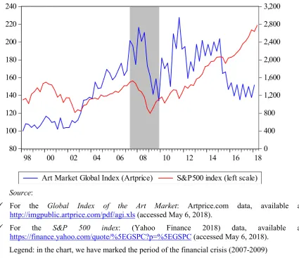
4 The dynamics of the S&P500 index and the Global Index of the Art Market (Artprice) are shown in the following figure below.

Figure 1. The dynamics of the S&P500 index and the Global Index of the Art Market (Artprice index)

Source:

 For the Global Index of the Art Market: Artprice.com data, available at http://imgpublic.artprice.com/pdf/agi.xls (accessed May 6, 2018).

 For the S&P 500 index: (Yahoo Finance 2018) data, available at https://finance.yahoo.com/quote/%5EGSPC?p=%5EGSPC (accessed May 6, 2018).

Legend: in the chart, we have marked the period of the financial crisis (2007-2009)

According the standard unit root tests [Augmented Dickey-Fuller (ADF), GLS transformed Dickey-Fuller (DFGLS), Phillips-Perron (PP), Kwiatkowski, et. al. (KPSS), Elliot, Richardson and Stock (ERS) Point Optimal, and Ng and Perron (NP)], both the global index of the art market and the

S&P500 index are nonstationary series. The single point break unit root tests lead to the same conclusion. But the Lee-Strazicich unit root test with one or two structural breaks (Lee and Strazicich 2003) reject the unit root under the hypothesis of two structural breaks at 10% for Global Index of the Art Market

and at (near) 10% for S&P500 index.

As methodology, we analysed the causal relationship between the two index, through Toda-Yamamoto version of Granger causality test. To estimate the relationship between the Artprice Global Art Market Index and the S&P 500 index we used a following relationship:

artt = α(S&P 500)t + f(t) + et,

where art is the Artprice Global Art Market Index, S&P500 stand for the S&P 500 financial market index, f (t) is a trend (linear, or nonlinear) function, e - error variable, t – time index (quarterly intervals for 1998 to 2018q1). Model allows for trend breaks (i.e. coefficients variability by periods).

80 100 120 140 160 180 200 220 240

0 400 800 1,200 1,600 2,000 2,400 2,800 3,200

98 00 02 04 06 08 10 12 14 16 18

(3)

5 2. The Causality Relationship between Art Market and Financial Market

Since, according to standard unit root tests, both the global index of the art market and the

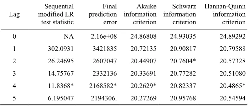
S&P500 index are nonstationary series, more exactly, I(1), we tested the presence of a causality relationship through Toda-Yamamoto version of Granger causality test. By using VAR Lag Order Selection Criteria to estimate the lag structure of VAR model, we found the following outputs:

Table 1. VAR Lag Order Selection Criteria

Endogenous variables: Global Index of the Art Market and S&P500 index Exogenous variables: C

Sample: 1998Q1 2018Q1 Included observations: 74

Lag

Sequential modified LR test statistic

Final prediction error

Akaike information criterion

Schwarz information criterion

Hannan-Quinn information criterion

0 NA 2.16e+08 24.86808 24.93035 24.89292

1 302.0931 3421835 20.72135 20.90817 20.79588

2 26.24695 2607047 20.44907 20.7604* 20.57328

3 14.75767 2332136 20.33691 20.77282 20.51080 4 11.8368* 2168582* 20.2629* 20.82337 20.4865*

5 6.195047 2194306. 20.27269 20.95768 20.54594

* indicates lag order selected by the criterion

Source: Estimates based on the Artprice.com and S&P 500 data (see Source of Figure 1).

Most criteria (4 of 5) have selected l = 4, so we built an VAR(4) model. According to Toda-Yamamoto methodology, in VAR(4) model we include, as exogenous, the variables with lag=5. In this model, we apply the VAR Granger Causality/Block Exogeneity Wald Tests. The outputs are the following:

Table 2. Testing causality relationship between S&P 500 and Global Index of the Art Market

Hypothesis Probability

S&P 500 does not Granger cause Global Index of the Art Market 0.0312

Global Index of the Art Market does not Granger cause S&P 500 0.8099

Source: Estimates based on the Artprice.com and S&P 500 data (see Source of Figure 1).

(4)

6 period (2007-2010). Even if it is an interesting result, however the causality test does not specify the sign of the causal relationship.

3. Exponential-Quadratic Model with Structural Breaks

To test the hypothesis that the art market is an alternative to securing (covering) financial investment in times of crisis, we have estimated the model

artt = α(S&P500)t + f(t) + et,

where we exogenously imposing two breaks (this is because Lee-Strazicich test reject the unit roots under the assumption of two structural breaks). If this hypothesis (the Art Market is an alternative for the Financial Market) is correct, then the coefficient α is negative, at the least in times of crisis (2007-2009). A weaker assumption is that α is non-significant, that is, there is no relationship between Art Market and Financial Market.

As trend function, f(t), we used an exponential-quadratic form: f(t) = a∙exp(t/10) + bt2_,

where a and b are coefficients that will be estimated through the model, along with α (in formula, we divided t to 10 only for scale reasons). This structure of the trend function was selected given the shape of the relationship between the two variables.

The outputs of the model estimation are as follows:









t /10 2

t t

(5.851) (2.627) ( 1.756) (4.848)

t /10 2

t

t t

( 1.861) (2.086) ( 2.762) (2.490)

for 1998Q1 to 2007Q2

70.6615 0.0261 S & P500

1.2377e

0.0944 t

u

for 2007Q3 to 2009Q4

art

_{786.135 0.1058 S & P500}

_9.6357e

_{0.8919 t}

_u

for 2010Q1 to



 









_

_

_

_





t /10 2

t t

(9.365) (4.839) ( 2.799) ( 3.880)

2018(Q1)

158.7303 0.1138 S & P500

0.0203e

0.0404t

u

 









_

_

_



(t-statistic in parenthesis, bellow the estimators).

As estimation method, we used Least Squares with Fixed Breaks (2007Q3 and 2010Q1). Also, we have inserted into the model, as non-breaking variables, the dummy for 2010Q4 and 2011Q3.

(5)

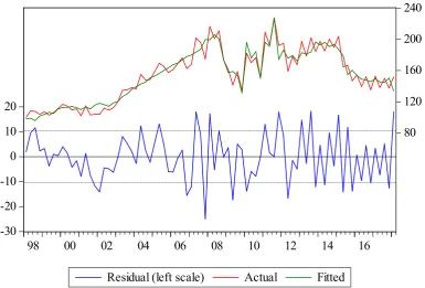
7 Figure 2. The relationship between global index of the art market and the S&P 500 index.

Econometric nonlinear (exponential-quadratic) model with Structural Breaks.

Source: Estimates based on the nonlinear (exponential-quadratic) model with Structural Breaks.

The model explains 92.1% of the art market index variation from its mean (according to R-squared) and all the coefficients are significant at the standard level of 5%. Errors are not autocorrelated (according to the Breusch-Godfrey Serial Correlation LM Test) and are not heteroscedastic (according to the White Heteroskedasticity Test). The model as a whole is significant: Prob (F-statistic = 60.432) <0.000001.

For all periods (before the crisis, in the time of crisis, and in post-crisis) the link between the dynamics of the Global Index of the Art Market and the evolution of the S&P 500 index (the coefficient α in the model) is significant and positive. The positive value of correlation signifies that the Global Index of the Art Market and the S&P 500 index evolve, as a trend, in the same way, which means that the art market has not been widely used as an alternative to the capital market, not even during the crisis.

4. Long-run Relationship between Art Market and Financial Market

If we assuming that both the short-run (VAR) dynamics and the cointegrating equations do not exhibit of intercept or linear trends, then we find a significant long-run equilibrium relationship between the Global Index of the Art Market and the S&P 500 index. For this purpose, we built a Structural Vector Error Correction (SVEC) model with 4 lags (according with the results presented in Table 1, above). In the Structural VEC Model, we imposed that all significant (at least at 10%) coefficients from non-structural model are zero. As well, we inserted, as exogenous in the equation of short-run dynamics, the eighth lag (two years) of the differentiated endogenous variable [namely, d(yt-8), where y is the exogenous variable].

The Structural VEC Model estimates are the following:

d(artt) = – 0.0403∙(artt-1 – 0.0616∙S&Pt-1) –

– 0.0012∙d(artt-1) + 0.1957∙d(artt-2) – 0.3049∙d(artt-3) + 0.0902∙d(artt-4) + -30

-20 -10 0 10 20

80 120 160 200 240

98 00 02 04 06 08 10 12 14 16

(6)

8 + 0.1829∙d(artt-8) + 0.0151∙d(S&Pt-1) + 0.0144∙d(S&Pt-2) + dummy + ut.

To simplify the writing, we use "art" to symbolize Global Index of the Art Market and "S&P" for S&P 500 index. In above equation, d is the operator of differencing and ut is the residual variable. The "dummy" stands for the dummy exogenous variables, selected by detecting the outliers in residual variable [more exactly, d(art2008q1), d(art2010q1), d(art2011q1)].

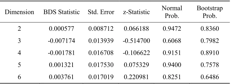
The SVEC model fit well the data: R2_{= 0.8186 and the residual variable does not contain a} linear, non-linear, or chaos structural patterns. According to the BDS (Brock, et al. 1996), the residuals of SVEC model are i.i.d. (independent and identically distributed): the probabilities associated with null hypothesis (the errors are i.i.d.) are greater than 5%, whatever is the embedding dimension for 2 to 6 (2 ≤ m ≤ 6). For that matter, the minimum of those probabilities is 64.86%, suitable to the correlation dimension equal to 6 (m = 6).

Table 3. BDS independence test for residuals in SVAR model.

Dimension BDS Statistic Std. Error z-Statistic Normal Prob.

Bootstrap Prob.

2 0.000577 0.008712 0.066188 0.9472 0.8360

3 -0.007174 0.013939 -0.514700 0.6068 0.7982

4 -0.001781 0.016708 -0.106622 0.9151 0.8910

5 0.001321 0.017530 0.075329 0.9400 0.7578

6 0.003761 0.017019 0.220981 0.8251 0.6486

Source: Estimates in EViews 10, based on the SVEC model.

For the SVEC model, the cointegration coefficient, β = – 0.0403, is negative and significantly different from zero (t-Statistic = -2.729).

The long-run relationship (equilibrium) between the Global Index of the Art Market and the

S&P 500 index arises in the first line of the equation:

art = 0.0616 S&P.

Written with the signification of the symbols, the long-run relationship is as follows:

Global Index of the Art Market = 0.0616 (S&P 500 index)

(7)

9 Conclusions

We tested the relationships between the Artprice Global Index of the Art Market and the S&P 500 index. If the Art market would be an alternative for the Financial market, then there should be a weak correlation between art market dynamics and the evolution of traditional asset classes. By applying the Toda-Yamamoto version of Granger causality test, we find that S&P 500 index may be a cause for

Global Index of the Art Market, but, the inverse causality relationship can be rejected: Global Index of the Art Market does not Granger cause S&P 500. These causality relationships are verified both for the whole analysed period (1998-2018q1) and in times of financial crisis (2007-20010).

Using a non-linear (exponential-quadratic) econometric model with structural breaks, we find that, for all periods (before the crisis, in the time of crisis, and after the crisis) the link between the dynamics of the Global Index of the Art Market and the evolution of the S&P 500 index is significant and positive. The positive value of correlation means that the Global Index of the Art Market and the

S&P500 index move, as a trend, in the same way, which shows that the art market has not been widely used as an alternative to the capital market, not even during the crisis.

We built, also, a Structural Vector Error Correction (SVEC) model for the purpose of analysis the long-run relationship between the Global Index of the Art Market and the S&P 500 index. The SVEC model outcomes show that, in the long-run, there is a positive relationship between the Global Index of the Art Market and the S&P 500 index, and these results confirm the conclusions of the econometric nonlinear (exponential-quadratic) model with structural breaks.

Bibliography

[1] Artprice. 2018. The Art Market in 2017. Annual Report, Artprice.com. Accessed May 6, 2018. https://www.artprice.com/artprice-reports/the-art-market-in-2017.

[2] Artprice. 2018. “The Contemporary Art Market Report 2017.” Saint-Romain-au-Mont-d'Or, France. Accessed February 16, 2018. https://www.artprice.com/artprice-reports/the-contemporary-art-market-report-2017/renewed-growth.

[3] Brock, William, Davis Dechert, Jose Sheinkman, and Blake LeBaron. 1996. “A Test for Independence Based on the Correlation Dimension.” Econometric Reviews 15 (3): 197-235. [4] Campbell, Rachel A.J. 2005. Art as an Alternative Asset Class. LIFE Research Paper No.

WP05-001, Maastricht: Maastricht University. http://ssrn.com/abstract=675643.

[5] Candela, Guido, and Antonello Eugenio Scorcu. 1997. “A Price Index for Art Market Auctions. An application to the Italian Market of Modern and Contemporary Oil Paintings.” Journal of Cultural Economics 21: 175-196.

[6] Codignola, Federica. 2015. “The Globalization of the Art Market: A Cross-Cultural Perspective where Local Features meet Global Circuits.” Chap. 5 in Analyzing the Cultural Diversity of Consumers in the Global Marketplace, by Juan Miguel Alcántara-Pilar, Salvador del Barrio-García, Esmeralda Crespo-Almendros and Lucia Porcu, 82-100. Hershey, PA: IGI Global.

[7] David, Géraldine, Kim Oosterlinck, and Ariane Szafarz. 2013. “Art market inefficiency.” Economics Letters 121 (1): 23-25.

[8] Ghinsburgh, Victor A. 2001. The Economics of Art and Culture. Amsterdam: Elsevier.

[9] Gilles, Dave. 2011. Testing for Granger Causality. 29 April. Accessed May 6, 2018. http://davegiles.blogspot.com/2011/04/testing-for-granger-causality.html.

[10] Goetzmann, William N, Luc Renneboog, and Christophe Spaenjers. 2010. “Art and Money.” NBER Working Paper No. 15502.

(8)

10 [12] Hutter, Michael, and David Throsby. 2008. Beyond Price. Value in Culture, Economics and the

Arts. Cambridge: Cambridge University Press.

[13] Jula, Dorin, and Nicolae Marius Jula. 2013. “Economic Growth and Structural Changes in Regional Employment.” Romanian Journal of Economic Forecasting (Institute for Economic Forecasting) 16 (2): 52-69.

[14] Jula, Dorin, and Nicolae-Marius Jula. 2018. Econometrie. Bucharest: Mustang.

[15] Kräussl, Roman, Thorsteh Lehnert, and Nicolas Martelin. 2017, June. 15th. “The True Value of Art.” True Value of Art Conference. Luxembourg: University of Luxembourg.

[16] Lee, Junsoo, and Mark C Strazicich. 2003. “Minimum Lagrange Multiple Unit Root Test With Two Structural Breaks.” Review of Economics and Statistics (MIT Press) 85 (4): 1082-1089. [17] Mamarbachi, Raya, Marc Day, and Giampiero Favato. 2008. “Art as an Alternative Investment

Asset.” 26 March. Accessed May 6, 2018. Available at SSRN: https://ssrn.com/abstract=1112630 or http://dx.doi.org/10.2139/ssrn.1112630.

[18] Mei, Jianping, and Michael Moses. 2002. “Art as an Investment and the Underperformance of Masterpieces.” NYU Finance Working Paper No. 01-012. 31 May. Accessed May 6, 2018. Available at SSRN: https://ssrn.com/abstract=311701 or http://dx.doi.org/10.2139/ssrn.311701. [19] Picinati di Torcello, Adriano, and Cyrielle Gauvin. 2017. Art as an Asset. Riga Graduate School

of Law. Riga (Latvia): Riga Graduate School of Law, 24 July. Accessed March 15, 2018. http://www.artlaw.online/en/read-it/articles/art-as-an-asset.

[20] Pownall, Rachel A.J. 2007. “Art as a Financial Investment.” 5 April. Accessed May 6, 2018. Available at SSRN https://ssrn.com/abstract=978467 or http://dx.doi.org/10.2139/ssrn.978467. [21] S&P Global. 2017. “S&P Down Jones Indices.” Index Mathematics. Methodology. S&P Global.

November. Accessed February 17, 2018.

https://www.spindices.com/documents/methodologies/methodology-index-math.pdf.

[22] The Wall Street Journal. 2018. Market Data Center. Accessed February 18, 2018. http://www.wsj.com/mdc/public/page/2_3022-djiahourly.html?mod=mdc_uss_pglnk.

[23] Toda, Hiro Y, and Taku Yamamoto. 1995. “Statistical inference in vector autoregressions with possibly integrated processes.” Journal of Econometrics 66 (1-2): 225-250.

[24] Velthuis, Olav. 2013. “Globalizaton of Market for Contemporary Art.” European Societies 15 (2): 290-308. Accessed May 6, 2018. doi:https://doi.org/10.1080/14616696.2013.767929.

[25] Yahoo Finance. 2018. S&P 500. Accessed June 9, 2018. https://finance.yahoo.com/quote/%5EGSPC?p=%5EGSPC.