www.astesj.com
Stabilization of constrained uncertain systems by an o
ff
-line
approach using zonotopes
Walid Hamdi*, Wissal Bey, Naceur Benhadj Braiek
Laboratory of Advanced Systems (L.A.S), Polytechnic School of Tunisia, Carthage University, BP 743,2078 La Marsa, Tunisia
A R T I C L E I N F O A B S T R A C T
Article history:
Received: 30 November 2017 Accepted: 07 January 2018 Online: 31 January 2018 Keywords:
Stabilization
Zonotopic invariant sets Model Predictive Control Uncertain systems
In this paper, stabilization of uncertain systems was established using zonotopic sets. The obtained state feedback control laws are computed by an off-line approach reducing computational burdens. The resolution of a robust model predictive control (MPC) allows computing a sequence of state feedback control laws corresponding to a sequence of zonotopic invariant sets. The implemented control laws are then calculated by lin-ear interpolation between the state feedback gains corresponding to the nested pre-computed zonotopic sets. The proposed interpolation with the use of zonotopic sets achieves better control performances.
1
Introduction
Model predictive control (MPC) is one of the most successful techniques of advanced control in the pro-cess industry. Thanks to the recent developments of the underlying theoretical framework, MPC has become a mature control technique able to provide controllers ensuring stability, robustness, constraint satisfaction and tractable computation for linear and nonlinear systems [1]. The MPC is can be made in the context of representation in state variables [2]. This not only make use of existing theorems and results in the state space theory, but also facilitates the exten-sion of the theory of model predictive control to more complex cases such as systems with stochastic distur-bances, noise on measured variables or multivariable control. For nonlinear uncertain systems, explicitly modeling of the uncertainty is essential [3].
For modeling uncertain systems, it is very impor-tant for MPC to be more robust [2]. Imporimpor-tant areas in MPC that have recently seen significant theoreti-cal and implementational progress include robust and stochastic MPC as well as efficient computations for MPC via convex and reliable real-time optimization [4].
Although these MPC schemes have remarkable performance and good theoretical properties, there is a hard computational burden due to the min-maximization of the optimization problem, especially in the presence of the system nonlinearity. The other
is to derive robust stability of MPC by minimization of linear quadratic optimization problems subject to polytopic uncertainty models and linear matrix in-equality (LMI) constraints, which was firstly proposed in [5]. From this formulation, a broad class of model uncertainty descriptions can be addressed with guar-anteed closed-loop robust stability of MPC.
Since the Lyapunov theory was introduced as an efficient stability analysis tool of systems governed by ordinary differential equations, the notion of set in-variant was used in many problems concerning the analysis and control of dynamic systems. An impor-tant motivation, leading to introduce invariant sets, was the need to analyze the effect of uncertain sys-tems. An invariant set is a region of the state space such the trajectory generated by the dynamical system remains confined in the set if the initial condition lies within it [6]. Robust controlled invariant set is partic-ularly relevant since it can be used in the context of constrained uncertain systems stability [7].
In recent years, in the theory of control, regard-less of a particular area, there have been numerical solutions are extensive. That is, a problem is usually considered as solved whenever it can be written as a (constrained) optimization problem. The difficulty in solving such a problem is greatly influenced by the way the constraint set is defined. In this context, sev-eral families of sets vie for influence [8].
Historically, ellipsoidal sets [9] were a useful choice of invariant sets due to their simple definition.
*Corresponding Author: Laboratory of Advanced Systems (L.A.S),Polytechnic School of Tunisia,+21641594777 &
Then, the problem becomes to design the invariant el-lipsoids off-line [10]. Recently, polyhedral sets [11], became widespread due to their representation flexi-bility and reliable numerical algorithmes. Angeli [12] proposed an ellipsoidal off-line MPC scheme for un-certain polytopic systems. In [13] the authors pro-posed an off-line robust constrained MPC algorithm by choosing a sequence of states.
However, polyhedral sets become numerically un-stable for higher dimensions and certain operations scale badly with respect to the complexity of the set in question. Zonotopic sets, a subclass of polyhedral sets [11], have started to gain attention. Their sym-metric shape, coupled with the flexibility inherited from the polyhedral class makes them an appealing choice for higher dimensions. Also, for dynamical sys-tems, zonotopes provide an excellent compromise be-tween accuracy and efficiency as first [14]. As a direct consequence, researchers from disparate fields started to employ them in various applications [15,16]. The greater part of this application exploits the zonotope facility in defining robust approximations.
Zonotopes are also used to rigorously estimate the states of dynamical systems as an alternative to ob-servers that optimize with respect to the best estimate, such as Kalman filters. One of the first works that use zonotopes for state-bounding observers is [17] and bounded disturbance in [18]. Similarly to reachabil-ity analysis, this work has been extended to nonlinear systems in [19,20] and systems with uncertain param-eters [21].
This paper is organised as follows, a description of the considered problem is first presented. Then, the optimal control problem for constrained uncer-tain systems is formulated. Its resolution procedure using zonotopic invariant sets with an interpolation step, is proposed. The efficiency of the used zonotopic invariant sets is then illustrated by two examples. Fi-nally, the paper is concluded.
2
Problem description
The considered system is the following linear time-varying (LTV) system with polytopic uncertainty:
x(k+ 1) =A(k)x(k) +Bu(k)
y(k) =Cx(k) (1)
wherex(k) is the state of the plant,u(k) is the control input andy(k) is the plant output. We assume that:
[A(k), B(k)]∈Ω,
Ω=conv{[A1, B1],[A2, B2], ...,[AL, BL]} (2)
whereconv is the convex hull and Omega is a poly-tope, [Aj, Bj] are vertices of the polytope such that:
h Aj, Bj
i
=
L
X
j=1
λj
h Aj, Bj
i ,
L
X
j=1
λj= 1,0≤λj≤1, (3)
The aim is this research is to find a state-feedback con-trol law:
u(k+i/k) =Kx(k+i) (4)
that stabilizes (1) with the following performance cost:
min
u(k+i/k)[A(k+i),Bmax(k+i)]∈Ω,i≥0J∞(k)
J∞(k) = ∞
P
i=0
"
x(k+i/k)
u(k+i/k)
#T"
Θ 0 0 R
# "
x(k+i/k)
u(k+i/k)
#
(5) subject to :
|uh(k+ 1/k)| ≤uh,max, h= 1,2, ..., nu (6)
yr(k+ 1/k)
≤yr,max, r= 1,2, ..., ny (7)
whereΘ >0 andR >0 are symmetric weighting ma-trices.
In [13] the authors describe the concept of an asymptotically stable invariant ellipsoid to develop a robust constrained MPC algorithm. This algorithm gives a sequence of explicit control laws correspond-ing to a sequence of asymptotically stable invariant ellipsoids constructed off-line one within another in state space. They solved, at each time step, the ro-bust constrained MPC problem using Linear Matrix Inequalities (LMI). The obtained result is considered conservative due to invariant ellipsoids which are an approximation of the real invariant sets.
In [5] the authors describe polyhedral invariant sets with an off-line robust algorithm to stabilize un-certain systems. They are calculated off-line a se-quence of state feedback control laws corresponding to a sequence of polyhedral invariant sets. At each sampling time, the smallest polyhedral invariant set that the currently measured state can be embedded is determined. The corresponding state feedback con-trol law is then implemented to the process.
We intend to use this algorithms with zonotopic representation of the invariant sets followed by an in-terpolation step to get less conservative results.
3
Robust MPC Algorithm
In this section, an interpolation-based robust MPC algorithm for uncertain polytopic discrete-time sys-tems using zonotopic invariant sets is presented. The nested zonotopic invariant sets and feedback gains are pre-computed off-line in first step, in order to reduce the on-line computational burdens. In second step, the real-time control law is calculated by linear in-terpolation between the feedback gains correspond-ing to the zonotopic invariant sets previously gener-ated. The optimization problem solved at each time step is based on optimization of linear performance index and only a computationally low-demanding op-timization problem is required to be solved on-line.
Definition 1:(Invariant sets)
such that for all x0 ∈ Ω, and all admissible input function u: R→U, the solution to system (1) with x(0) =x0satisfiesx(t)∈Ωfor allt≥0.
Intuitively, the system remains trapped in the in-variant for all future times [22].
One of the advantages of invariant sets, compared with iterative methods, is that they cover unbounded time horizon, without any extra cost. A second one is that they that have in general a compact represen-tation. For example, an invariant ellipsoid is repre-sented by a single nn matrix. Whereas, iterative meth-ods produce a large number of sets, often with grow-ing complexity. Each of these sets has to be taken into account in order to enclose all reachable states.
3.1
O
ff
-line Steps
Step 1: Choose a state sequencexi, i∈ {1,2, ..., N}and
solve the following problem to obtain corresponding state feedback gains:
Ki=YiQ
−1
i (8)
The states xi must be chosen such that the distance
betweenxi+1 and the origin is less than the distance betweenxiand the origin. MatricesYiandQ
−1
i , for all
i= 1,2, ..., Nare solutions of the following problem:
min
γi,Qi,Yi
γi (9)
subject to:
"
1 xTi xi Qi
#
≥0, (10)
Qi QiATj +YTBTj QiΘ1/2YiTR1/2
AjQi+BjYi Qi 0 0
Θ1/2Qi 0 γiI 0
R1/2Yi 0 0 γiI
≥0 (11)
∀j= 1,2, . . . , L
"
X Yi
YiT Qi
#
≥0, Xhh≤u2
h,max, h= 1,2, . . . , nu (12)
"
S C(AjQi+BjYi)
(AjQi+BjYi)TCT Qi
#
≥0, Srr≤yr,2max,
r= 1,2, . . . , ny, ∀j= 1,2, . . . , L,
(13)
Step 2: Given the state feedback gains:
Ki =YiQ
−1
i , i∈ {1,2, . . . , N} (14)
from step 1. For eachKi, the corresponding
polyhe-dral invariant sets defined by:
Si={xi/Mixi≤di} (15)
are constructed by the following :
Step 2.1: Set Mi =
h
CT,−CT, KT
i ,−KiT
iT , di =
h
ymaxT , yminT , umaxT , uminT
iT
andm= 1.
Step 2.2: Select row m from (Mi, di) and check
whether Mi,m(Aj+BjKi)x≤di,mis redundant with
re-spect to the constraints defined by (Mi, di) by solving
the problem:
max
x Wi,m,j (16)
subject to
Wi,m,j=Mi,m(Aj+BjKi)x−di,m, Mix≤di (17)
Step 2.3: Let m=m+ 1 and return to Step 2.2. If m is strictly larger than the number of rows in (Mi, di)
then terminate.
3.2
On-line Step using polyhedral sets
3.2.1 Without interpolation
At each sampling time, determine the smallest poly-hedral invariant set Si = {xi/Mixi ≤di} where i =
1,2, ..., N−1.
containing the measured states and implement the corresponding state feedback control law u(k/k) =
Kix(k/k) to the process.
3.2.2 With 3-points interpolation
At each sampling time, if the measured state lies be-tweenSi, Si+1andSi+2, i= 1,2, ..., N−1 implement the interpolated gain obtained by :
K =α1Ki−2+α2Ki−1+α3Ki (18)
where 0< αi<1,for alli= 1,2,3 and
3
P
i=1
αi = 1.
3.3
On-line Step using zonotopic sets
Zonotopes are convex polytopes that are centrally symmetric. Equivalently, a zonotope is a Minkowski sum of a finite set of line segments. A polytope is a zonotope if it can also be represented by so-called generators (G-representation).
Definition 2:(G-representation of a zonotope) Given a vectorc ∈Rn and a set of vectors ofRn,G= {g1, ..., gm}, m≥n, a zonotopeZof order m is defined as following:
Z=
x∈Rn, x=c+
p
X
i=1
γi.gi;−1≤γi ≤1
(19)
The vector c is called the center of the zonotope Z. The vectorsg1, ..., gmare called generators ofZ.
The order of zonotope is defined by the number of its generators (min this case). In the case of m < n, its called degenerated zonotope.
This definition is equivalent with the definition of zonotopes by the Minskowski sum of a finite number of line segments defined bygiB1. Z= (c;g1, g2, ..., gm) =
c⊕g1B1⊕...⊕gmB1WhereBnis a unitary box inRn, is a box composed by n unitary intervals. And⊕is the Minkowski sum.
The Minkowski sum of two sets X and Y is defined by
X⊕Y={x+y:x∈X, y∈Y}. Definition 4:(Unitary interval)
The unitary interval is defined byBn= [−1,1]. Definition 5:(Box)
A box is an interval vector. An interval hull of a set
Z⊆Rn , denoted byZis a box that satisfiesZ⊆ Z Given a boxZ = ([a1, b1], ...,[an, bn])T. mid(Z), de-notes its center anddiam(Z) = (b1−a1, ..., bn−an)T Definition 6:(Unitary box)
A unitary box, denoted byBnis a box compound byn
unitary intervals.
Definition 7:(V-representation of a polytope) Givenrverticesvi∈Rn,P =conv{v1, ..., vr}is a convex
polytope, where conv is the convex hull operator. To obtain zonotopic sets from polyhedral ones, we have to perform the following three steps:
Step 1: Compute the vertices vi ∈ Rn
(V-representation) of all N polytopesSi, i= 1, , N.
Step 2:Obtain the minimum and maximum values of each polytopei:
mmin= min(Vi1, ..., Viv),
mmax= max(Vi1, ..., Viv).
(20)
whereVijis theithcomponent ofvjandris the num-ber of the vertices of each polytope.
Step 3: Compute a G-representation of the n-dimensional interval [mmin, mmax] :
[mmin, mmax] =
x=c+Xn
i=1γi.gi,−1≤γi≤1
,
(21) where :
c= 0.5(mmin+mmax), (22)
gi(i)=
(
0.5(mmax−mmin), if i=j
0, otherwise (23)
3.3.1 Without interpolation
At each sampling time, determine the smallest invari-ant zonotope
Z=
(
x|x=c+
p
P
i=1
γi.gi,−1≤γi≤1
)
, i= 1,2, ..., N−1
containing the measured states and implement the corresponding state feedback control law u(k/k) =
Kix(k/k) to the process.
3.3.2 With 2-points interpolation
At each sampling time, if the measured state lies be-tweenZi and Zi−1, implement the interpolated gain obtained by :
K=αKi+ (1−α)Ki+1 (24)
where 0< αi<1, for alli= 1,2, and
2
P
i=1
αi= 1.
3.3.3 with 3-points interpolation
At each sampling time, if the measured state lies be-tweenZi,Zi−1 and Zi−2, implement the interpolated gain obtained by:
K=α1Ki−2+α2Ki−1+α3Ki (25)
where 0< αi<1,for alli= 1,2,3, and
3
P
i=1
αi = 1.
4
Application
In this section, we are going to present two examples allowing to implement the proposed approach. For both examples, the software Yalmip toolbox [23] in the MATLAB environment was used to compute the solution of the LMI minimization problem.
4.1
Example 1
Lets consider an uncertain non-isothermal CSTR [5] where the exothermic reaction AB takes place. The reaction is irreversible and the rate of reaction is first order with respect to component A. A cooling coil is used to remove heat that is released in the exothermic reaction. The uncertain parameters are: the reaction rate constantk0 and the heat of reaction∆Hrxn. The
linearized model based on the component balance and the energy balance is given by the following state equations:
(
x(t+ 1) =A(t)x(t) +B(t)u(t)
y(t) =Cx(t) (26)
where x =
" CA
T #
is the state vector x(t) and u =
" CA,F
FC
#
is the control input vectoru(t). Matrices are
defined by:
A=
−F
V −k0e
−E/RTs − E
RTs2k0e −E/RTs
CAs
−∆Hrxnk0e−E/RTs
ρCp
−F
V −V ρCU Ap −∆Hrxn E
ρCpRTs2k0e −E/RTs
CAs
(27)
B=
F
V 0
0 −2.098×10⁵Ts−365
V ρCp
, (28)
C=
"
1 0
0 1
#
(29)
Where CA is the concentration of A in the
reac-tor, C(A,F) is the feed concentration of A, T is the reactor temperature, and FC is the coolant flow.
The operating parameters are: F = 1m3/min, V = 1m3, k0= 109−1010min
−1
, ER = 8330.1K,−∆Hr×n = 107 − 108cal/kmol, ρ = 106g/m3, U A = 5.34 × 10⁶cal/(kmin)and Cp= 1cal/(gk). LetCA=CA−CA,eq,
TA=T−Teq,CA,F=CA,F−CA,F,eq andFC=FC−FC,eq
discrete-time model with
" CA(k)
T(k)
#
as a state vector
and
"
CA,F(k)
FC(k)
#
as a control vector, is given as follows:
(
x(k+ 1) =A(k)x(k) +B(k)u(k)
y(k) =Cx(k) (30)
where:
A=
"
0.85−0.0986α(k) −0.0014α(k) 0.9864α(k)β(k) 0.0487 + 0.01403α(k)β(k)
#
B=
"
0.15 0 0 −0.912
#
, C=
"
1 0 0 1
#
(31) where: 1 ≤ α(k) = k0/109 ≤ 10 and 1 ≤ β(k) = −∆Hrxn/107≤10.
The two parameters (k) and (k) are independent of each other. Then, we consider the following polytopic uncertain model with four vertices:
Ω=Co
"
0.751 −0.0014 0.986 0.063
# ,
"
0.751 −0.0014 9.864 0.189
# ,
"
0.751 −0.0014 0.986 0.063
# ,
"
0.751 −0.0014 9.864 0.189
# ,
(32) The objective is to regulate the concentrationCAand
the reactor temperature T to the origin by manip-ulating CA,F and FC , respectively. These variables
are constrained by:C
A,F
≤ 0.5kmol/m
3, and FC
≤
1.5m3/min.
The cost function is given by (5) with Θ = I and
R= 0.1I.
Lets choose a sequence of states:
xi=
(0.0525,0.0525),(0.0475,0.0475),
(0.0425,0.0425),(0.0375,0.0375),
(0.0325,0.0325),(0.0275,0.0275)
(33)
This sequence is used to calculate six off-line feedback gainsKi, i= 1,2, ...,6. The regulated output (the
con-centration of A and the reactor temperature), when
α(k) and β(k) are randomly time-varying between 109≤α(k) = 1010and 107≤β(k) =∆H
r×n≤108. The obtained zonotopes are defined by:
ci=
n
2.98,3.17,−1.31,1.31,−3.17,−2.98 o, (34)
Whereci is the center of the zonotopeZi,i= 1,2, ..,6.
The generators matrices are defined by:
gi=
3.07 0 0 0 0 0
0 3.26 0 0 0 0
0 0 1.29 0 0 0
0 0 0 1.29 0 0
0 0 0 0 3.26 0
0 0 0 0 0 3.07
(35)
for alli= 1,2, ..,6.
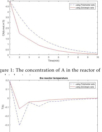
The regulated outputs are shown respectively in Fig-ure 1 and FigFig-ure 2. It is seen that the considered zono-topic sets give less conservative results and better sys-tem performance as compared to the approach using polyhedral ones.
Figure 1: The concentration of A in the reactor of the regulated output
Figure 2: The reactor temperature of the regulated outputIn Figure 3 and Figure 4 respectively, it is seen
that the considered interpolation using three zono-topic sets, give less conservative results as compared to the approach with interpolation of polyhedral sets.
Figure 3: The concentration of A in the reactor of the regulated output
4.2
Example 2
We consider the angular positioning system [4]. It consists of an electric motor driving a rotating an-tenna so that it always points in the direction of a moving object. The motion of the antenna can be de-scribed by the following discrete time-equation:
" θ(k+ 1)
•
θ(k+ 1)
#
=
"
1 0.1 0 1−0.1α(k)
# " θ(k)
•
θ(k)
#
+
"
0 0.0787
# u(k)
y(k) = [1 0]
" θ(k)
•
θ(k)
#
(36)
whereθ(k) is the angular position of the antenna, •
θ(k) is the angular velocity andu(k) is the input voltage of the motor. It is assumed that the uncertain parameter is arbitrarily time-varying : 0.1α(k)10.
Letθ=θ−θeq, • θ= • θ− • θ
eqandu=u
−ueqwhere the
sub-scripteqdenotes the corresponding variable at equi-librium condition. The obtained system can be writ-ten as follows:
θ(k+ 1) •
θ(k+ 1)
= "
1 0.1 0 1−0.1α(k)
#
θ(k) •
θ(k)
+ " 0 0.0787
# u(k)
y(k) = [1 0]
θ(k) •
θ(k)
(37)
The system (36) has the following polytopic struc-ture:
A(k)∈conv ("
1 0.1 0 0.9
# ,
"
1 0.1 0 0
#)
(38)
The input constraint is:
|u(k)| ≤2volts (39)
The weighting matricesΘandRare given by:
Θ=
"
1 0 0 0
#
and R= 0.00002I (40)
Lets choose the following sequence of seven states:
xi=
(0.35,0.35),(0.3,0.3),
(0.25,0.25),(0.02,0.02),
(0.15,0.15),(0.1,0.1),(0.05,0.05)
(41)
This sequence is used to calculate seven state feedback gainsKi corresponding to seven polyhedral invariant
sets. The obtained zonotopes are defined by their cen-ters:
ci =
(
1.52,−0.08,−0.21,0.21, 0.08,−1.52,0.21
)
i= 1,2, ...,7. (42)
The zonotope generators are given by:
gi=
0.82 0 0 0 0 0 0
0 3.87 0 0 0 0 0
0 0 0.70 0 0 0 0
0 0 0 3.38 0 0 0
0 0 0 0 0.59 0 0
0 0 0 0 0 2.87 0
0 0 0 0 0 0 0.47
(43) for alli= 1,2, ...,7.
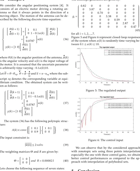
Figure 5 and Figure 6 represent closed-loop responses of the system whenα(k) is randomly time-varying be-tween 0.1≤α(k)≤10.
Figure 5: The regulated output
Figure 6: The control input
We can observe that by the considered approach with zonotopic sets using three points interpolation especially the one with three control gains, we obtain better control performances as compared to the ap-proach with interpolation of polyhedral sets.
5
Conclusion
addition, an interpolation step to the obtained control laws based on polyhedral and zonotopic invariant sets respectively was employed. The proposed approach applied on examples showed that the control perfor-mance using zonotopic invariant sets followed by an interpolation of the nested zonotopes is better than the one using polyhedral invariant sets.
References
1. S. Kheawhom and P. Bumroongsri. Interpolation-based ro-bust constrained model predictive output feedback control, in Conference on Control and Automation. June 16-19. Palermo, Italy, 2014.
1. B. Ding, Y. Xi, M. T. Cychowski and T.O.Mahony. Improving off-line approach to robust MPC based-on nominal perfor-mance cost, Automatica, vol. 43, No. 1, pp. 158163, 2007.
2. X. Liu, S. Feng and M. Ma, Robust MPC for the constrained system with polytopic uncertainty. International Journal of Systems Science, vol. 43, No. 2, pp. 248258, 2012..
3. F. Borelli. Constrained optimal control of linear and hybrid systems, vol 290 of Lecture Notes in Control and Informa-tion Sciences, Springer, 2010.
4. M. H. Nehrir, C. Wang, Modeling and Control of Fuel Cells: Distributed Generation Applications, Wiley-IEEE Press, 2009.
5. B. Pornchai and K. Soorathep. An off-line robust MPC al-gorithm for uncertain polytopic discrete-time systems using polyhedral invariant sets, Journal of Process Control, vol.22, No. 5, pp. 975-983, 2012.
6. F. Blanchini and S. Miani.Set-theoretic methods in control. Systems and Control, Foundations and Applications, 2008.
7. A. Bemporad. M. Morari, V. Dua. and E. N. Pistikopoulos. The explicit linear quadratic regulator for constrained sys-tems, Automatica, vol. 38, pp. 3-20, 2002.
8. W. Bey, Z. Kardous and N. Benhadj Braiek. Stabilization of Constrained uncertain systems by Multi-Parametric Op-timization,International Journal of Automation and Con-trol(IJAAC), vol. 10, n. 4, pp. 407-416, Inderscience En-terprises Ltd, 2016.
9. A. B. Kurzhanskii and I. Vlyi. Ellipsoidal calculus for es-timation and control, Burlhauser, Boston, Massachusets, 1997.
10. A. C. Brooms, B. Kouvaritakis, and Y. I. Lee. Constrained MPC for uncertain linear systems with ellipsoidal target sets, Systems and Control Letters, vol. 44, No. 3, pp. 157166, 2011.
11. A. Matthias, S. Olaf and B. Martin. Computing reachable sets of hybrid systems using a combination of zonotopes and polytopes, Nonlinear Analysis: Hybrid Systems, vol.4, No. 2,pp. 233-249, 2010.
12. A. Casavola, D. Angeli, G. Franze and E.Mosca. An ellip-soidal off-line MPC scheme for uncertain polytopic discrete-time systems, Automatica, vol. 44, No. 12, pp. 31133119, 2008.
13. Z. Wan and M. V. Kothare, An efficient off-line formulation of robust model predictive control using linear matrix in-equalities. Automatica, vol. 39, No. 5, pp. 837846, 2003.
14. A. Ingimundarson, J. M. Bravo, V. Puig, T. Alamo and P. Guerra. Robust fault detection using zonotope-based set-membership consistency, International journal of adaptive control and signal processing, vol. 23, No. 4, pp. 311330, 2008.
15. M. Althoff, O. Stursberg and M. Buss. Computing reachable sets of hybrid systems using a combination of zonotopes and polytopes, Nonlinear Analysis: Hybrid Systems, vol. 4, No. 2, pp. 233249, 2010.
16. J. Blesa, V. Puig and J. Saludes. Identification for passive ro-bust fault detection using zonotope-based set-membership approaches, International Journal of Adaptive Control and Signal Processing, vol.25, No.9, pp. 788-812, 2011. 17. C. Combastel. A state bounding observer based on
zono-topes, In Proceeding of the European Control Conference, 2003.
18. F. Stoican, S. Olaru, J. A. De Don and M. M. Seron. Zono-topic ultimate bounds for linear systems with bounded dis-turbances, In Proceedings of the 18th IFAC World Congress, Milano, Italy, pp. 92249229, 2011.
19. T. Alamo, J. M. Bravo and E. F. Camacho. Guaranteed state estimation by zonotopes, In Proceeding of the 42nd IEEE Conference on Decision and Control, pp. 58315836, 2003. 20. C. Combastel. A state bounding observer for uncertain
nonlinear continuous-time systems based on zonotopes, In Proceeding of the 44th IEEE Conference on Decision and Control, and the European Control Conference, ECC, pp.72287234, 2005.
21. V. T. H. Le, C. Stoica, T. Alamo, E. F. Camacho and D. Du-mur. Zonotopic guaranteed state estimation for uncertain systems. Automatica, vol. 49, No. 11, pp.4183424, 2013. 22. I. Ben Makhlouf, P. Hansch and S. Kowalewski.
Compar-ison of Reachability Methods for Uncertain Linear Time-Invariant Systems, European Control Conference (ECC) July 17-19 Zrich, Switzerland, 2013.