A Direct Matrix Inversion-Less Analysis for Distribution System Power Flow Considering Distributed Generation

1- Introduction

Almost in all topics relevant to expansion, operation, and management of DSs, it is very important to solve the power flow problem as efficient and simple as possible. The traditional power flow algorithms are not suitable for DSs. Therefore, several algorithms for solving distribution power flow problem have been proposed. These algorithms based on basic approaches which have been used to construct them can be classified into three categories: (a) methods based on Newton-Raphson (NR) and Newton-like methods, (b) backward/forward sweep methods (BFSMs) and (c) DMs. To modify conventional power flow methods, NR-based methods have initially been suggested to solve ill-conditioned power systems [1]-[3]. Then, methods based on general meshed topology such as transmission systems have been proposed [4]-[8]. A branch-current based NR approach has been proposed in [9]. Fast decoupled Newton methods for DSs have been developed in [10]-[12]. In recent years, current injection methods (CIMs) based on current injection equations have been proposed [13]-[15]. Generally speaking, these methods lack the advantages of simple implementation and low computations since they have not explicitly exploited characteristics of DSs.

BFSMs based on network topology of DSs are very prevalent due to their promising performance and simplicity in implementation [16]-[23]. The main idea of these methods has been suggested in [16] in which a new power flow method for the calculation of branch current flows has been proposed using compensation based technique and Kirchhoff’s laws. Future developments of BFSMs for real-time analysis with an The corresponding author; Email: [email protected]

emphasis on modeling of unbalanced and distributed loads in [19], and the extension version allowing modeling of voltage-dependent loads in [20] have been presented. In [24], the newest BFSM is presented and it is claimed that this method is faster and more flexible than the other BFSMs. One of the main disadvantages of BFSMs is poor convergence for WMDSs [25].

The third category was based on formation of an impedance matrix and solving equations in the form of V=ZI [26]-[29]. The method which can express the voltage of each load in terms of load’s currents and common impedances of the loads for RDSs has been proposed in [26]. In [27]-[28], the author develops two matrices to express bus voltages as a function of branch currents, line parameters, and the substation bus voltage. In recent years, two new DMs have been presented [30]-[31] but matrix inversion is needed by such methods. The DMs as will be shown in the simulation results have a better performance over the two other methods. However, they have not been fully developed. They only solve meshes at the end of feeders and, moreover, it is not clear how they deal with different models of loads. Moreover, in some papers, DMs use additional features to solve meshes which decrease their efficiency.

This paper presents a new direct power flow method trying to deal with the above issues. The main advantages of the proposed method are I) its robustness and efficiency upgraded considerably since it is no longer necessary to use matrix inversion- being the main reason of divergence and low-efficiency of the power flow algorithms, b) its capability to solve meshes as efficiently and simply as RDSs where only a current ratio is used, c) its capability to solve DSs, even including more than one mesh.

AUT J. Elec. Eng., 50(1)(2018)85-92 DOI: 10.22060/eej.2017.11646.4984

A Direct Matrix Inversion-Less Analysis for Distribution System Power Flow

Considering Distributed Generation

A. Mahmoudi1*_{, S. H. Hosseinian}2_{, H. Zarabadipour}3

1 _{Department of Electrical Engineering, Takestan Branch, Islamic Azad University, Takestan, Iran.} 2 _{Electrical Engineering Department, Amirkabir University of Technology Tehran, Iran.}

3 _{Department of Technical & Engineering, Imam Khomeini International University, Qazvin, Iran}

ABSTRACT: This paper presents a new direct matrix inversion-less analysis for radial distribution systems (RDSs). The method can successfully deal with weakly meshed distribution systems. (WMDSs). Being easy to implement, direct methods (DMs) provide an excellent performance. Matrix inversion is the mean reason of divergence and low-efficiency in power flow algorithms. In this paper, the performance of the proposed DM is upgraded since it is no longer necessary to use the matrix inversion and its related computations. On the other hand, DMs have not been explicitly developed for different models of loads and, moreover, analyzing meshes in previous works decreases the efficiency of such methods. This paper deals with these issues and takes a few steps forward. The modeling of distributed generations in distribution systems is also studied which is an interesting topic nowadays. Simulations results for balanced, unbalanced, meshed and radial systems with distributed generations verify the performance of the proposed method.

Review History:

Received: 17 May 2016 Revised: 6 October 2017 Accepted: 6 November 2017 Available Online: 5 December 2017

Keywords:

can deal with different models of loads and meshes. However, they usually use NR-based methods to solve DSs because of shortcomings of BFSMs and DMs. Therefore, they lack advantages of DMs such as simplicity of implementation, low computations, and robustness.

The present paper is organized as it follows. First, the proposed method is developed for RDSs in Section 2 where different models of loads are also studied. Modification of the proposed method for WMDSs is presented at Section 3. DG Modeling restricted to PQ mode is studied in Section 4. In the end, test results are presented in Section 5.

2- Algorithm Development for RDSs

The radial characteristic of DSs can be used to solve them as simple circuits. Consider a DS, including only a radial main feeder as shown in Figure 1. If the ladder iterative technique suggested by [30] is used for this feeder, after some manipulation, the voltage of load i at k-th iteration can be obtained by

1 1 1

1

(

1

...

)

k k k k k

i i i i i n

V

V

z I

−

I

−

I

−

− +

=

−

+

+ +

(1) where z_i is impedance of the branch located between load i-1 and load i, and I_ik-1 _{is the current injection of bus i at (k-1)-th} iteration.

I

1

V

s

I

2

I

i

I

n

z

1

V

1

z

2

V

2

V

i

V

n

Figure 1: Single line diagram of a simple main distribution feeder

The voltage of bus 1 with respect to the substation bus voltage (V_s) and current injections can be expressed as:

1 1 1

1k s 1 1

(

k 2k

...

nk

)

V

= −

V z I

−

+

I

−

+ +

I

− ₍₂₎

Repeating the same process for other buses yields the following formula as

1 1

i n

k k

i s r j

r j r

V

V

z I

−

= =

=

−

∑∑

(3) The unknown values in (3) can be restricted to current injections if V_i is expressed in terms of I_i and the equivalent load impedance of bus i. To apply such simplification and obtain the equivalent load impedance, the model of loads connected to bus i must be considered as [32]:

a) Constant power loads

for such loads, V_i can be written as:

(

2 _*

)

/

i Pi Pi i Pi Pi

V Z I

=

=

V

S I

, (4) where Z_Pi, I_Pi, and S_Pi are the equivalent impedance, current and power of the constant power load connected to bus i, respectively.

b) Constant impedance loads

the impedance of such loads is constant, so V_i can be written as

i Zi Zi

V Z I

=

, (5)

where Z_Zi and I_Zi are the impedance and the current of the constant impedance load connected to bus i, respectively. c) Constant current loads

in this model, the magnitude of load current and also the current injection of bus i are constant. Therefore, the number of unknown values (current injections) is decreased; hence, the equation of V_i can be neglected. However, the phase of the current of such load changes to keep the power factor constant, it must be updated at each iteration as

(

)

Ci Ci i i

I

=

I

∠

δ θ

−

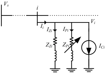
(6) where I_Ci and θ_i are the current and power factor angle of the constant current load connected to bus i, respectively. Note that δ_i denotes the phase of V_i.

i

Z

Zi

Z

Pi

I

_Ci

I

Zi

I

Pi

V

s

V

i

I

i

Figure 2: A bus with three models of loads or a combination load

d) Combination loads

a combination load can be modeled by assigning a percentage of the total load to each of the three mentioned models. The total line current entering the load is the sum of the three components as shown in Figure 2 [32]. In this condition, the equivalent load’s impedance, current, and voltage of bus i can be calculated as

Z_Li = Z_Pi||Z_Zi (8) I_i = I_Pi+I_Zi+I_Ci (7) V_i = Z_Li (I_i-I_Ci) (9) Consequently, in general case, equation (3) after some manipulation can be rewritten as:

1

(

)

s ij

n

k k k k

Li i Ci j

j

V

Z I

I

Z I

=

−

= −

∑

, i=1,…,n (10) where Z_ij is the common impedance between bus i and j. It is the summation of line impedances through them current injections of bus i and j flow together. The formation and characteristics of this Z matrix are the same as that given in [26]. Equation (10) after some manipulation can be expressed in matrix form for all buses as

(

[ ] [

k

] [ ] [ ] [

)

k k

][

k

]

L s L C

that the equivalent load impedances are much greater than the line impedances. Therefore, it can be written as

[Z][Ik_]

<< [ZLk][Ik] (12)

Using (12) and this fact that the difference of current injections at two consecutive iterations is too small, an accurate approximation can be obtained as

1

([ ] [

k

])[ ] [ ][

k k

] [

k

][ ]

k

L L

Z

+

Z

I

≅

Z I

−

+

Z

I

. (13) This approximation has no effect on the accuracy of the proposed method as clearly explained in simulation results. Now current injections can be obtained from (11) and (13) as

(

)

1 1

[ ] [

k k

] [ ] [

k

][ ] [ ][

k k

]

L s L C

I

=

Z

−

V

+

Z

I

−

Z I

− ₍₁₄₎

1

[

k

]

[ ]

k

L L

Z

−

=

Y

(15) where Y_L is a n×n square diagonal matrix and its main diagonal elements represent equivalent load admittances. It is clear that such admittances are the reverse of equivalent load impedances. This simplicity of inversion is the direct result of this fact that Z_L is a square diagonal matrix; therefore, Y_L can be calculated by reversing the main diagonal elements of Z_L. As can be seen in (14) and (15), the matrix inverting operation is no longer required in the proposed method which makes the method performance more superior to others. In fact, the main reason of divergence, time-consuming and heavy computations in power flow algorithms is related to the calculation of matrix inverse. Therefore, this elimination can be considered as a great contribution in DS analyses.

Up to now, the proposed DM has been presented. The outline of the algorithm is to solve (16) through (19) iteratively,

2 _*

/

k k

Pi i Pi

Z

=

V

S

i=1,2,..,n (16)

(

)

k k

Ci Ci i i

I

=

I

∠

δ

−

θ

i=1,2,..,n (17)

(

1

)

[ ] [ ] [ ] [

k k k

][

k

] [ ][

k

]

L s L C

I

=

Y

V

+

Z

I

−

Z I

−

(18)

[ ] [ ]

1

k k

s

V

+

V

Z I





=

−

 





 

(19)

It can be seen that only the equivalent load impedances of constant power loads and the phase of the current of constant current loads are variable and must be updated at each iteration. The proposed method can easily be expanded to solve the three-phase power flow problem where the line impedances and current injections must be presented with 3×3 matrices and 3×1 vectors, respectively.

3- Algorithm Development for WMDSs

Normally closing open tie-switches creates a few meshes in DSs and such switches introduces WMDSs; however, the number of such meshes is restricted and WMDSs have been discussed often with one mesh in the literature. In this section, a new method for solving DSs with one mesh is proposed. The proposed method is applied to the meshes independently from their locations and is as efficient and simple as RDSs. Also, it can deal with more than one mesh in DSs.

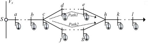
To solve WMDSs as simple as RDSs, the solution of RDSs is applied to WMDSs. In radial feeders, current injection paths are completely defined but when a mesh is created, some of the current injections can flow through two paths as shown in Figure 3, e.g. I_k can flow through Path1 and Path2. In fact, to apply RDS solution, in this case, the proportions of each

current injection in the two paths must be specified. If these proportions are specified, considering the electrical circuit theory, the voltage drops of different paths, through which a bus is fed, are the same. Consequently, to calculate the voltage of each bus, one of such paths is selected and swept. In order to calculate current proportions, assume that current injections of the buses located on the mesh flow completely through their paths (e.g. current injections of d and e flow completely through Path1 and current injections of f and g flow completely through Path2). It should be noted that the end of meshes can change in such a way that this assumption would always be correct. Also, assume that the current proportions of the buses located after the mesh flowing through Path1 and Path2 are α₁ and α₂, respectively (e.g. α₁(I_h + I_k + … + I_l) flow through Path1 and α₂(I_h + I_k + … + I_l) flow through Path2). Now the remaining problem is to calculate α₁

or α₂. Three methods are suggested for this purpose and are presented in the following.

a b c

d e

f g

h k

Vs

Path1

Path2

S l

Figure 3: One line diagram of a central mesh

3- 1- Current divider rule

If current injections of the buses located on the mesh can be neglected, then the current divider rule can be used to calculate α₁(α₂), e.g. in Figure 3, it can be calculated as

1

z

Path2

/ (

z

Path1

z

Path2

) 1

2

α

=

+

= −

α

(20) where z_Path1 and z_Path2 are the impedances of Path1 and Path2. 3- 2- KVL method

The Kirchhoff’s Voltage Law (KVL) can be applied to the mesh to calculate α₁ (α₂). The nominal values of the current injections are used to solve the KVL equation. This method is also approximate; however, it is more accurate than the current divider rule.

3- 3- Auxiliary equation method

ahead, z_xy is the impedance of a line(s) connecting bus x to bus y. Path1 is swept to calculate voltage drops of the buses located after the mesh.

A) If bus i is located before the mesh, the calculation process will be the same as that in RDSs, i.e.

ij ji Sa i a Sb i b Sc i c

Z

=

Z

=

z

=

or z

=

or z

= (21)

B) If bus i is located on the mesh, there are two conditions as: a) bus j is also located on the mesh.

i. If two buses are located on the same path e.g. Path1 (i = d, j = e), their current injections flow completely through the line between c and d, thus,

ij ji Sc cd

Z

=

Z

=

z

+

z

(22) ii. If two loads are located on different paths (i = d & j = f ), there is no common impedance between current injections on the mesh, thus,

ij ji Sc

Z

=

Z

=

z

(23) b) If bus j is located after the mesh, there are two conditions as:

i. If bus i is located on the selected path, Path1,(e.g. i = d) I_i flows completely through the line between c and d, but the proportion of I_j flowing through this line is α₁, i.e. current proportions of bus i and j flowing through the line between c and d are 1 and α₁, respectively, then,

1

ij Sc cd

Z

=

z

+

α

z

(24)

ji Sc cd

Z

=

z

+

z

(25) ii. If bus i is located on the other path, Path2, (e.g. i = f),

I_i does not flow through the line between c and d but the current proportion of bus j flowing through the line between c and f is α₂, then,

2

ij Sc cf

Z

=

z

+

α

z

(26)

ji Sc

Z

=

z

. (27) C) If both buses are located after the mesh (i = k, j = l), their current proportions flowing through Path1 are α₁, then,

1 1

ij ji Sc Path hk

Z

=

Z

=

z

+

α

z

+

z

(28) It can be seen that the changes were easily applied to the Z matrix and this matrix lost its symmetry for WMDSs. There is no need to change the solution process to analyze WMDSs and, moreover, the method is as efficient and simple as that of RDSs. As can be seen, the proposed method uses no additional features which may decrease its efficiency to analyze meshes. 4- Distributed Generation Modeling

In recent years, distributed generations (DGs) become more popular and the total installed capacity of such sources has grown drastically. These are usually used in constant power factor mode due to the fact that the standards prohibit active voltage regulation [33]-[34]. In this mode, when the active powers of them are specified, DGs can be modeled as PQ-buses.

It is clear when a DG is connected to the network, it sends current in reverse direction regarding the loads. Therefore, the only modification to study DGs in the proposed method is to consider their power injections with minus sign.

5- Simulation Results

In this section, first the three main categories of power flow algorithms are compared and then the accuracy of the proposed method for WMDSs is verified. In the end, a network with two meshes and a DG is analyzed to show the ability of the method. The proposed method was implemented within the MATLAB computing environment using Intel® Pentium® Dual-Core Desktop Processor E5200, 2.5 GHz and 2GB memory. The convergence tolerance is set at 0.0001 p.u. 5- 1- Comparison of the three main methods

As mentioned in Introduction, several methods based on the three main categories have been presented to solve DSs. In [13] and [25], it was shown that the performance of the CIMs is better than that of other NR methods and BFSMs. The BFSM suggested by [24] is also selected as the representative of BFSMs. Among DMs, the method suggested by [27] has a better performance than the others’ and must be studied.

Figure 4: A 90-bus radial distribution feeder

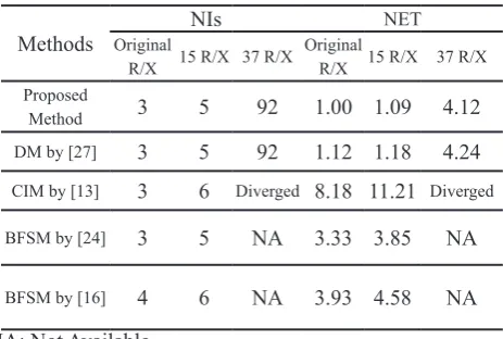
Case I: Bus with Extreme Radial Topology: First the 90-bus test system with extreme radial topology shown in Figure 4 and taken from [24] is studied. Important computational parameters which must be compared are Number of Iterations (NIs) and Normalized Execution Time (NET). Table 1 gives the results of such parameters for this practical feeder.

Table 1: Results of computations for Case 1

Methods Original NIs NET

R/X 15 R/X 37 R/X Original R/X 15 R/X 37 R/X Proposed

Method 3 5 92 1.00 1.09 4.12

DM by [27] 3 5 92 1.12 1.18 4.24

CIM by [13] 3 6 Diverged 8.18 11.21 Diverged

BFSM by [24] 3 5 NA 3.33 3.85 NA

BFSM by [16] 4 6 NA 3.93 4.58 NA

NA: Not Available

GHz, respectively, and the PC memories are the same). Table 1 shows that the performance of DMs is better than that of the other methods. There is no considerable difference between NIs but the two DMs are almost four times faster than the others. On the other hand, when the initial values of the R/X ratios are increased to verify the robustness of the methods, the proposed DM converged until 37×(R/X) even though the voltage of bus 7 was as low as 0.4718 p.u. However, this factor is equal to 28 for the CIM, and it is not specified for BFSM by [24]. Therefore, in addition to the simplicity and time-saving, the robustness is another advantage of the DMs. The two DMs have almost the same performances. The DM presented by [27] only calculates the voltage drop of each bus voltage, and the load characteristics are not considered. Moreover, only a simple method for the constant power loads is presented. However, in this paper, the load voltages are converted to the equivalent load impedances which simplify the simulating of different models of loads. In fact, one of the main advantages of the proposed method is to simplify the method suggested by [27] to simulate different load models while its performance is not affected.

L1 L2

V

s

L3 L4 L6 L7 L8 L9

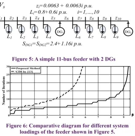
zi=0.0063 + 0.0063i p.u.

Li=0.8+0.6i p.u. i=1,…,10

DG1 DG2

SDG1=SDG2=2.4+1.16i p.u.

z1 z2 z3 z4 z5 z6 z7 z8 z9 z10

Figure 5: A simple 11-bus feeder with 2 DGs

1 2 3 4 5 6 7 8 9

0 5 10 15 20 25 30

β

Num

be

r o

f I

ter

ati

ons

Proposed Method CIM by [13]

Figure 6: Comparative diagram for different system loadings of the feeder shown in Figure 5.

Case II: 11-Bus With Two DG Simple Radial Feeder: To study a simple radial feeder including DGs, a simple feeder shown in Figure 5 is studied. DGs have not modeled in [16], [27] & [24]. To verify the robustness of the proposed method, the initial values of the loads and R/X ratios of this feeder were gradually increased up to the point where convergence was no longer attained. The NIs required to find the solution when all loads were varied by factor β is shown in Figure 6. Figure 7 shows the performance of the methods when the initial R/X ratios of the branches were increased by factor γ. It can be seen that the proposed method is numerically robust and requires fewer iterations than the CIM. In Figure 6, when each load is increased up to 9.4 times, convergence is still attained in the proposed method. This value is equal to 6.6 in the CIM.

Case III: Three-Phase Study: IEEE 37 Node Test Feeder: To study three-phase power flow, the IEEE 37 Node Test Feeder shown in Figure 8 is studied. This feeder is highly unbalanced and has three models of loads. Its loads are

connected in the delta but in this study, they are considered line-to-ground. Moreover, regulator and the transformer connecting node 709 to 775 are not implemented in this paper. In order to verify the robustness of the proposed method as case II, the same process is applicable in this study. Figures 9 and 10 show the effect of different system loadings and R/X ratios on NIs. The same conclusions can be derived in this case where studies show the robustness and fast convergence of the proposed DM.

2 4 6 8 10 12 14 16 18 0

5 10 15 20 25 30

γ

N

um

be

r o

f I

te

ra

tio

ns

Proposed Method CIM by [13]

Figure 7: Comparative diagram for different R/X ratios of the feeder shown in Figure 5.

Figure 8: IEEE 37 Node Test Feeder

2 4 6 8 10 12 14 16

0 5 10 15 20 25 30

β

N

um

be

r o

f I

te

ra

tio

ns

Proposed Method CIM by [14]

Figure 9: Comparative diagram for different system loadings of the IEEE 37 Node Test Feeder

nonzero terms must be constructed in the BFSM suggested by [24]. Then, this RCM must be inverted to construct a Section Bus Matrix (BSM) and, moreover, the BSM must be transported to construct another required matrix (Bus Section Matrix). In CIM proposed in [13], a 178×178 Jacobian matrix must be constructed and the inverse of this matrix must be calculated at each iteration. On the other hand, the number of Jacobian matrix elements which must be updated at each iteration is equal to 4×45 for the CIM while it is only 45 for the proposed method.

2 4 6 8 10 12 14 16 18 20

0 5 10 15 20 25 30

γ

N

um

be

r o

f I

te

ra

tio

ns

Proposed Method CIM by [14]

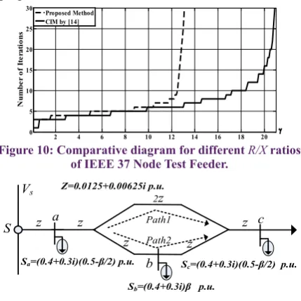
Figure 10: Comparative diagram for different R/X ratios of IEEE 37 Node Test Feeder.

a

b

c Vs

Path2

S z z Path1 z

z z

2z

Z=0.0125+0.00625i p.u.

Sa=(0.4+0.3i)(0.5-β/2) p.u.

Sb=(0.4+0.3i)β p.u.

Sc=(0.4+0.3i)(0.5-β/2) p.u.

Figure 11: A feeder with one mesh (the worst case study)

10 20 30 40 50 60 70 80 90

0 1 2 3 4 5 6 7 x 10-3

β(%)

M

ax

im

um

e

rro

rs

Current divider rule method KVL method ×100 Auxiliary equation method×100

Figure 12: Maximum errors of the proposed method when the load imbalance on the two paths shown in

Figure 11 is increased by factor β (%)

Vs

10

I1

I3

I4

I5 I6

Si=0.4+0.3i p.u. i=1,…,6 except 2

2 7 8

SDG=-1.2-0.58i p.u.

DG

9

Figure 13: A system with two meshes and a DG

5- 2- WMDS Study

Different studies on the accuracy of the proposed method for WMDSs show that the worst case occurs when there is a high load imbalance on the two paths of the mesh. The feeder shown in Figure 11 is studied to simulate such conditions

where loads are centralized at three points and total loads are constant. That portion of the load located on Path 2 is increased by the factor β while there is no load on Path 1. In other words, the percentage of the load imbalance on the two paths is increased. Figure 12 shows maximum errors of the proposed method when the three methods are used to calculate α₁ (α₂).

It should be noted that the maximum errors of the KVL and auxiliary equation methods are multiplied by 100 in Figure 12. As can be seen in this figure, the maximum errors of these two methods are much smaller than the convergence tolerance in all conditions. The maximum errors in the current divider rule method are also smaller than the convergence tolerance upto 15% load imbalance and it is restricted to 0.007 p.u. in complete load imbalance (when all loads are located on Path 2). Moreover, the feeder loadings in Figure 11 are heavy, thus, the voltage of bus c drops to 0.96 p.u. Hence, the current divider rule method can be used for normal WMDSs when the load imbalance on the two paths is less than 15% of total loads. It is clear that most of the load imbalances of WMDSs are smaller than 15%. In severe cases, the KVL method can be used which always has a reasonable accuracy. Therefore, as shown in Figure 12, WMDSs are solved using only the current divider rule or the KVL for the mesh. There is no need to use the auxiliary equation method at all.

Table 2: Bus voltages of the system shown in Figure 13

Bus No. The proposed method CIM [13]

10 1.0000 1.0000

1 0.9863 0.9863

2 0.9787 0.9787

3 0.9765 0.9764

4 0.9765 0.9764

5 0.9754 0.9756

6 0.9783 0.9787

7 0.9804 0.9802

8 0.9881 0.9878

9 1.0049 1.0045

5- 3- Highly meshed DSs with penetration of DG

6- Conclusion

In this paper, a new DM for DS power flow analysis was developed. The proposed DM uses neither matrix inversion nor its related computations. It considers load characteristics by defining the equivalent load impedances which simplifies the simulating of different models of loads. It was shown that the proposed method is numerically very robust and requires fewer iterations. Moreover, the proposed DM has been developed for WMDSs using three simple methods for solving meshes. The performance of the proposed approach for WMDSs is as efficient and simple as RDSs. The results show that the present method is efficient and suitable for large-scale DSs.

References

[1] Iwamoto, S. and Y. Tamura. A load flow calculation method for ill-conditioned power systems, IEEE transactions on power apparatus and systems, 4 (1981)1736-1743. [2] Tripathy, S. and G. P. Prasad, Load flow solution for

ill-conditioned power systems by quadratically convergent Newton-like method. IEE Proceedings C (Generation, Transmission and Distribution), IET. 128 (1980) 250 – 251.

[3] Tripathy, S., et al. Load-flow solutions for ill-conditioned power systems by a Newton-like method, IEEE transactions on power apparatus and systems, 10 (1982) 3648-3657.

[4] Chen, T.-H., et al, Three-phase cogenerator and transformer models for distribution system analysis, IEEE Transactions on Power Delivery, 6 (1991) 1671-1681.

[5] Chen, T.-H., et al, Distribution system power flow analysis-a rigid approach, IEEE Transactions on Power Delivery, 6 (1991) 1146-1152.

[6] Birt, K. A., et al., Three phase load flow program, IEEE transactions on power apparatus and systems, 95 (1976) 59-65.

[7] Chen, T.-H. and J.-D. Chang, Open wye-open delta and open delta-open delta transformer models for rigorous distribution system analysis. IEE Proceedings C (Generation, Transmission and Distribution), IET. 139 (1992) 227 – 234.

[8] Teng, J.-H. and W.-M. Lin. Current-based power flow solutions for distribution systems. Proc. IEEE Int. Conf. Power Syst. Technol. 1994.

[9] Lin, W. and J. Teng, Phase-decoupled load flow method for radial and weakly-meshed distribution networks, IEE Proceedings-Generation, Transmission and Distribution, 143 (1996) 39-42.

[10] Zimmerman, R. D. and H.-D. Chiang, Fast decoupled power flow for unbalanced radial distribution systems, IEEE Transactions on Power Systems, 10 (1995) 2045-2052.

[11] Hatami, A. and M. M. PARSA, Three-phase fast decoupled load flow for unbalanced distribution systems, 6 (2007) 31-35.

[12] Rajicic, D. and A. Bose, A modification to the fast decoupled power flow for networks with high R/X ratios, IEEE Transactions on Power Systems, 3 (1988) 743-746. [13] da Costa, V. M., et al., Developments in the Newton

Raphson power flow formulation based on current injections, IEEE Transactions on Power Systems 14 (1999) 1320-1326.

[14] Garcia, P. A., et al., Three-phase power flow calculations using the current injection method, IEEE Transactions on Power Systems 15 (2000) 508-514.

[15] Penido, D. R. R., et al., Three-phase power flow based on four-conductor current injection method for unbalanced distribution networks, IEEE Transactions on Power Systems, 23 (2008) 494-503.

[16] Shirmohammadi, D., et al., A compensation-based power flow method for weakly meshed distribution and transmission networks, IEEE Transactions on Power Systems, 3 (1988) 753-762.

[17] Luo, G.-X. and A. Semlyen, Efficient load flow for large weakly meshed networks, IEEE Transactions on Power Systems, 5 (1990) 1309-1316.

[18] Cheng, C. S. and D. Shirmohammadi, A three-phase power flow method for real-time distribution system analysis, IEEE Transactions on Power Systems, 10 (1995) 671-679.

[19] Cespedes, R., New method for the analysis of distribution networks, IEEE Transactions on Power Delivery, 5 (1990) 391-396.

[20] Das, D., et al., Novel method for solving radial distribution networks, IEE Proceedings-Generation, Transmission and Distribution, 141 (1994) 291-298. [21] Haque, M., Efficient load flow method for distribution

systems with radial or mesh configuration, IEE Proceedings-Generation, Transmission and Distribution, 143 (1996) 33-38.

[22] Chang, G., et al., An improved backward/forward sweep load flow algorithm for radial distribution systems, IEEE Transactions on Power Systems, 22 (2007) 882-884. [23] Kumar, K. V. and M. Selvan, A simplified approach

for load flow analysis of radial distribution network, International Journal of Computer and Information Engineering, 2 (2008) 273-283.

[24] AlHajri, M. and M. El-Hawary, Exploiting the radial distribution structure in developing a fast and flexible radial power flow for unbalanced three-phase networks, IEEE Transactions on Power Delivery, 25 (2010) 378-389.

[25] Araujo, L., et al., A comparative study on the performance of TCIM full Newton versus backward-forward power flow methods for large distribution systems, IEEE PES Power Systems Conference and Exposition, 2006. [26] Goswami, S. and S. Basu, Direct solution of distribution

systems. IEE Proceedings C (Generation, Transmission and Distribution), 138 (1991) 78-88.

[27] Teng, J.-H., A direct approach for distribution system load flow solutions, IEEE Transactions on Power Delivery, 18 (2003) 882-887.

[28] Teng, J.-H., A network-topology-based three-phase load flow for distribution system, Source: Proceedings of the National Science Council, China, Part A: Physical Science and Engineering, 24 (2000) 259-264.

Please cite this article using:

A. Mahmoudi, S. H. Hosseinian, H. Zarabadipour, A Direct Matrix Inversion-Less Analysis for Distribution System Power Flow Considering Distributed Generation, AUT J. Elec. Eng., 50(1)(2018) 85-92.

DOI: 10.22060/eej.2017.11646.4984

load flow, IEEE Power Engineering Review, 20 (2000) 60-62.

[30] Mahmoudi, A. and S. H. Hosseinian, Direct solution of distribution system load flow using forward/backward sweep, 19th Iranian Conference on Electrical Engineering (ICEE), 2011.

[31] Mahmoudi, A., et al., A Novel Direct Power Flow for Distribution Systems with Voltage-Controlled Buses, Iranian Journal of Science and Technology, Transactions of Electrical Engineering, 42 (2018) 149-160.

[32] Kersting, W. H, Distribution system modeling and analysis, CRC press 2001.

[33] Basso, T. S. and R. DeBlasio, IEEE 1547 series of standards: interconnection issues, IEEE Transactions on Power Electronics, 19 (2004) 1159-1162.