Volume 2008, Article ID 578612,9pages doi:10.1155/2008/578612
Research Article
Auditory Sparse Representation for Robust Speaker
Recognition Based on Tensor Structure
Qiang Wu and Liqing Zhang
Department of Computer Science and Engineering, Shanghai Jiao Tong University, Shanghai 200240, China
Correspondence should be addressed to Liqing Zhang,[email protected]
Received 31 December 2007; Accepted 29 September 2008
Recommended by Woon-Seng Gan
This paper investigates the problem of speaker recognition in noisy conditions. A new approach called nonnegative tensor principal component analysis (NTPCA) with sparse constraint is proposed for speech feature extraction. We encode speech as a general higher-order tensor in order to extract discriminative features in spectrotemporal domain. Firstly, speech signals are represented by cochlear feature based on frequency selectivity characteristics at basilar membrane and inner hair cells; then, low-dimension sparse features are extracted by NTPCA for robust speaker modeling. The useful information of each subspace in the higher-order tensor can be preserved. Alternating projection algorithm is used to obtain a stable solution. Experimental results demonstrate that our method can increase the recognition accuracy specifically in noisy environments.
Copyright © 2008 Q. Wu and L. Zhang. This is an open access article distributed under the Creative Commons Attribution License, which permits unrestricted use, distribution, and reproduction in any medium, provided the original work is properly cited.
1. INTRODUCTION
Automatic speaker recognition has been developed into an important technology for various speech-based appli-cations. Traditional recognition system usually comprises two processes: feature extraction and speaker modeling. Conventional speaker modeling methods such as Gaussian mixture models (GMMs) [1] achieve very high performance for speaker identification and verification tasks on high-quality data when training and testing conditions are well controlled. However, in many practical applications, such systems generally cannot achieve satisfactory performance for a large variety of speech signals corrupted by adverse con-ditions such as environmental noise and channel distortions. Traditional GMM-based speaker recognition system, as we know, degrades significantly under adverse noisy condi-tions, which is not applicable to most real-world problems. Therefore, how to capture robust and discriminative feature from acoustic data becomes important. Commonly used speaker features include short-term cepstral coefficients [2, 3] such as linear predictive cepstral coefficients (LPCCs), mel-frequency cepstral coefficients (MFCCs), and perceptual linear predictive (PLP) coefficients. Recently, main efforts are focused on reducing the effect of noises and distortions.
Feature compensation techniques [4–7] such as CMN and RASTA have been developed for robust speech recognition. Spectral subtraction [8,9] and subspace-based filtering [10, 11] techniques assuming a priori knowledge of the noise spectrum have been widely used because of their simplicity.
Currently, the computational auditory nerve models and sparse coding attract much attention from both neuroscience and speech signal processing communities. Lewicki [12] demonstrated that efficient coding of natural sounds could provide an explanation for both the form of auditory nerve filtering properties and their organization as a population. Smith and Lewicki [13, 14] proposed an algorithm for learning efficient auditory codes using a theoretical model for coding sound in terms of spikes. Sparse coding of sound and speech [15–18] is also proved to be useful for auditory modeling and speech separation, providing a potential way for robust speech feature extraction.
value decomposition for tensor decomposition, which is a multilinear generalization of the matrix SVD. Vasilescu and Terzopoulos [20] introduced a nonlinear, multifactor model called Multilinear ICA to learn the statistically independent components of multiple factors. Tao et al. [21] applied general tensor discriminant analysis to the gait recognition which reduced the under sample problem.
In this paper, we propose a new feature extraction method for robust speaker recognition based on auditory periphery model and tensor structure. A novel tensor analysis approach called NTPCA is derived by maximizing the covariance of data samples on tensor structure. The benefits of our feature extraction method include the following. (1) Preprocessing step motivated by the auditory perception mechanism of human being provides a higher frequency resolution at low frequencies and helps to obtain robust spectrotemporal feature. (2) A supervised learning procedure via NTPCA finds the projection matrices of multirelated feature subspaces which preserve the individual, spectrotemporal information in the tensor structure. Fur-thermore, the variance maximum criteria ensures that noise component can be removed as useless information in the minor subspace. (3) Sparse constraint on NTPCA enhances energy concentration of speech signal which will preserve the useful feature during the noise reduction. The sparse tensor feature extracted by NTPCA can be further processed into a representation called auditory-based nonnegative tensor cepstral coefficients (ANTCCs), which can be used as feature for speaker recognition. Furthermore, Gaussian mixture models [1] are employed to estimate the feature distributions and speaker model.
The remainder of this paper is organized as follows. In Section 2, an alternative projection learning algorithm NTPCA is developed for feature extraction. Section 3 describes the auditory model and sparse tensor feature extraction framework. Section 4presents the experimental results for speaker identification on three speech datasets in the noise-free and noisy environments. Finally,Section 5 gives a summary of this paper.
2. NONNEGATIVE TENSOR PCA
2.1. Principle of multilinear algebra
In this section, we briefly introduce multilinear algebra and details can be found in [19,21,22]. Multilinear algebra is the algebra of higher-order tensors. A tensor is a higher-order generalization of a matrix. Let X ∈ RN1×N2×···×NM denotes a tensor. The order ofXisM. An element ofXis denoted by Xn1,n2,...,nM, where 1 ≤ ni ≤ Ni and 1 ≤ i ≤ M. The mode-i vectors of X are Ni-dimensional vectors obtained
fromXby varying indexniand keeping other indices fixed.
We introduce the following definitions relevant to this paper.
Definition 1(mode-dmatricizing). Let the ordered setsR= {r1,. . .,rL}andC= {c1,. . .,cK}be a partition of the tensors
N = {1,. . .,M}, whereM =L+K. The matricizing tensor can then be specified by
X(R×C)∈RL×K withL=
i∈R
Ni,K=
i∈C
Ni. (1)
The mode-d matricizing of an Mth-order tensor X ∈
RN1×N2×···×NM is a matrixX
d ∈ RL×K, whereL = Nd and
K = i /=dNi. The mode-d matricizing ofXis denoted as
matd(X) orXd.
Definition 2 (tensor contraction). The contraction of a tensor is obtained by equating two indices and summing over all values of the repeated indices. Contraction reduces the tensor order by 2. When the contraction is conducted on all indices except theith index on the tensor product ofXandY inRN1×N2×···×NM, the contraction result can be denoted as
X⊗Y;ii
=X⊗Y;1 :i−1,i+ 1 :M1 :i−1,i+ 1 :M
=
N1
n1=1 · · ·
Ni−1
ni−1=1
Ni+1
ni+1=1 · · ·
NM
nM=1
Xn1×···×ni−1×ni+1×···×nM
×Yn1×···×ni−1×ni+1×···×nM =mati(X)matTi(Y)
=XiYiT,
(2)
and [X⊗Y; (i)(i)]∈RNi×Ni.
Definition 3(mode-dmatrix product). The mode-dmatrix product defines multiplication of a tensor with a matrix in moded. LetX∈RN1×···×NMandA∈RJ×Nd. Then, theN
1×
· · · ×Nd−1×J×Nd+1× · · · ×NMtensor is defined by
X×dA
N1×···×Nd−1×J×Nd+1···×NM
=
Nd
XN1×···×Nd···×NMAJ×Nd
=X⊗A; (d)(2).
(3)
In this paper, we simplify the notation as
X×1A1×2A2× · · · ×AM=X M
i=1
×iAi, (4)
X×1A1× · · · ×i−1Ai−1×i+1Ai+1× · · · ×AM
=X
M
k=1,k /=i
×kAk=X×iAi. (5)
2.2. Principal component analysis with nonnegative and sparse constraint
The basic idea of PCA is to project the data along the directions of maximal variances so that the reconstruction error can be minimized. Let x1,. . .,xn ∈ Rd form a zero
mean collection of data points, arranged as the columns of the matrix X ∈ Rd×n, and letu
1,. . .,uk ∈ Rd be the
principal vectors, arranged as the columns of the matrixU∈
with nonnegative and sparse constraint is proposed, which is called NSPCA:
max
U
1 2 U
TX 2 F−
α 4 I−U
TU 2
F−β1TU1 s.t.U≥0,
(6)
whereA2
Fis the square Frobenius norm, the second term
relaxes the orthogonal constraint of traditional PCA, the third term is the sparse constraint, α > 0 is a balanc-ing parameter between reconstruction and orthogonality, β ≥ 0 controls the amount of additional sparseness required.
2.3. Nonnegative tensor principal component analysis
In order to extend NSPCA in the tensor structure, we change the form of (6) sinceA2
F =tr(AAT) andDefinition 3and
obtain following equation:
max
U≥0
1 2tr
UTXUTXT−α 4 I−U
TU 2
F−β1TU1
=max
U≥0
1 2tr
UT
n
i=1
XiXiT
U
−α 4 I−U
TU 2
F−β1TU1
=max
U≥0
1 2
n
i=1
Xi×1UT
⊗Xi×1UT
; (1)(1)
−α 4 I−U
TU 2
F−β1TU1.
(7)
LetXidenote theith training sample with zero mean which
is a tensor, and Uk is thekth projection matrix calculated
by the alternating projection procedure. Here,Xi (0 ≤i ≤
n) are r-order tensors that lie in RN1×N2×···Nr and U
k ∈
RNk∗×Nk (k = 1, 2,. . .,r). Based on an analogy with (7), we define nonnegative tensor principal component analysis by replacing Xi with Xi. So we can obtain the optimization
problem as follows:
max
U1,...,Ur≥0 1 2
n
i=1
Xi r
k=1
×kUkT
⊗ Xi r
k=1
×kUkT
; (1 :r)(1 :r)
−α 4
r
k=1 I−UT
kUk
2
F−β r
k=1
1TUk1.
(8)
In order to obtain the numerical solution of the problem defined in (8), we use the alternating projection method, which is an iterative procedure. Therefore, (8) is decomposed
intordifferent optimization subproblems as follows:
max
Ul≥0 (l=1,...,r)
1 2
n
i=1
Xi r
k=1
×kUkT
; ⊗ Xi r
k=1
×kUkT
(1 :r)(1 :r)
−α 4
r
k=1 I−UT
kUk
2
F−β r
k=1
1TUk1
= max
Ul≥0 (l=1,...,r)
1 2
n
i=1
Xi×lUlT×lUlT
⊗Xi×lUlT×lUlT
; (1 :r)(1 :r)
−α 4 I−U
T l Ul
2
F−β1 TU l1 −α 4 r
k=1,k /=l
I−UT
kUk 2F−β r
k=1,k /=l
1TU k1
= max
Ul≥0 (l=1,...,r)
1 2tr
UlT
n
i=1
matl
Xi×lUlT
×matTlXi×lUlT
Ul
−α 4 I−U
T
l Ul 2F−β1TUl1
−α 4
r
k=1,k /=l
I−UT kUk
2
F−β r
k=1,k /=l
1TUk1.
(9)
In order to simplify (9) we define
Al= n
i=1
matl
Xi×lUlT
matTlXi×lUlT
,
Cl= −α
4
r
k=1,k /=l
I−UT kUk
2
F−β r
k=1,k /=l
1TUk1.
(10)
Therefore, (9) becomes
max
Ul≥0 (l=1,...,r)
1 2 U
T l Bl
2
F−
α 4 I−U
T l Ul
2
F−β1 TU
l1+Cl,
(11)
where Al = BlBTl. But as described in [23], the above
optimization problem is a concave quadratic programming, which is an NP-hard problem. Therefore, it is unrealistic to find the global solution of (11), and we have to settle with a local maximum. Here we give a function of ul pq as the
optimization objective
ful pq
= −α 4u
4
Input:Training tensorXj∈RN1×N2×···Nr, (1≤j≤n), the dimensionality of the output tensors Yj∈RN
∗
1×N2∗×···Nr∗,α,β, maximum number of training iterationsT, error thresholdε. Output:The projection matrixUl≥0 (l=1,. . .,r), the output tensorsYj.
Initialization: SetUl(0)≥0 (l=1,. . .,r) randomly, iteration indext=1. Step 1. Repeat until convergence{
Step 2. Forl=1 tor { Step 3. CalculateA(lt−1);
Step 4. Iterate over every entries ofUl(t)until convergence
– Set the value oful pqto the global nonnegative maximizer of (12) by evaluating it over all nonnegative roots of
(14) and zero; }
Step 5. Check convergence: the training stage of NTPCA convergence ift > Tor update errore < ε
} Step 6. Yj=Xj
r l=1×lUl
Algorithm1: Alternating projection optimization procedure for NTPCA.
Speech Pre-emphasis Cochlear filters
Nonlinearity
DCT GMM
X
U
NTPCA
Recognition result
Cochlear feature
Feature tensor by different speakers
Spectral-temporal projection matrix
Figure1: Feature extraction and recognition framework.
where const is the independent term oful pqand
c1=
d
i=1,i /=q
alsiul pi−α· k
i=1,i /=p d
j=1,j /=q
ul p juli juliq−β,
c2=alqq+α−α· d
i=1,i /=q
u2l pi−α· k
i=1,i /=p
u2liq,
(13)
where ali j is the element ofAl. Setting the derivative with
respect toul pqto zero, we obtain a cubic equation
∂ f
∂ul pq = −αu
3
l pq+c2ul pq+c1=0. (14)
We calculate the nonnegative roots of (14) and zero as the nonnegative global maximum of f(ul pq). Algorithm 1
lists the alternating projection optimization procedure for Nonnegative Tensor PCA.
3. AUDITORY FEATURE EXTRACTION BASED ON
TENSOR STRUCTURE
The human auditory system can accomplish the speaker recognition easily and be insensitive to the background noise.
In our feature extraction framework, the first step is to obtain the frequency selectivity information by imitating the process performed in the auditory periphery and pathway. And then we represent the robust speech feature as the extracted auditory information mapped into multiple interrelated feature subspace via NTPCA. A diagram of feature extraction and speaker recognition framework is shown inFigure 1.
3.1. Feature extraction based on auditory model
We extract the features by imitating the process occurred in the auditory periphery and pathway, such as outer ear, middle ear, basilar membrane, inner hair cell, auditory nerves, and cochlear nucleus.
Because the outer ear and the middle ear together generate a bandpass function, we implement traditional pre-emphasis to model the combined outer and middle ear functions xpre(t) = x(t)−0.97x(t−1), where x(t) is the
discrete-time speech signal, t = 1, 2,. . ., andxpre(t) is the
1 0.5 0 −0.5 −1
A
m
plitude
0 0.5 1 1.5 2 2.5 3 3.5 4 Time (s)
(a) 3911
1914 857 321 50
Fre
q
u
en
cy
(H
z)
0 0.5 1 1.5 2 2.5 3 3.5 4 Time (s)
(b)
Figure2: Clean speech sentence and illustrations of cochlear power feature. Note the asymmetric frequency resolution at low and high frequencies in the cochlear.
The frequency selectivity of peripheral auditory system such as basilar membrane is simulated by a bank of cochlear filters. The cochlear filterbank represents frequency selectivity at various locations along the basilar membrane in a cochlea. The “gammatone” filterbanks implemented by Slaney [24] are used in this paper, which have an impulse response in the following form:
gi(t)=aitn−1e2πbiERB(fi)tcos
2π fit+φi
(1≤i≤N), (15)
where n is the order of the filter, N is the number of filterbanks. For theith filter bank, fiis the center frequency,
ERB(fi)=24.7(4.37fi/1000 + 1) is the equivalent rectangular
bandwidth (ERB) of the auditory filter, φi is the phase,
ai,bi ∈ R are constants, where bi determines the rate of
decay of the impulse response, which is related to bandwidth. The outputs of each gammatone filterbank is xi
g(t) =
τxpre(τ)gi(t−τ).
In order to model nonlinearity of the inner hair cells, we compute the power of each band in every frame k with a logarithmic nonlinearity
P(i,k)=log
1 +γ
t∈framek
xig(t)
2
, (16)
where P(i,k) is the output power, γ is a scaling constant. This model can be considered as average firing rates in the inner hair cells, which simulate the higher auditory pathway. The resulting power feature vector P(i,k) at frame k with component index of frequency ficomprises the
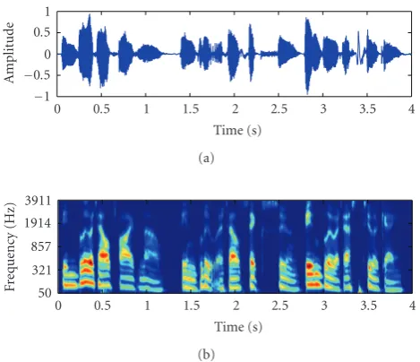
spectrotem-poral power representation of the auditory response.Figure 2 presents an example of clean speech utterance (sampling rate 8 kHz) and corresponding illustrations of the cochlear power feature in the spectrotemporal domain. Similar to mel-scale
processing in MFCC extraction, this power spectrum pro-vides a much higher frequency resolution at low frequencies than at high frequencies.
3.2. Sparse representation based on tensor structure
In order to extract robust feature based on tensor structure, we model the cochlear power feature of different speakers as 3-order tensorX∈RNf×Nt×Ns. Each feature tensor is an array with three modelsfrequency×time×speaker identitywhich comprises the cochlear power feature matrixX∈RNf×Nt of different speakers. Then we transform the auditory feature tensor into multiple interrelated subspaces by NTPCA to learn the projection matrices Ul (l = 1, 2, 3). Figure 3
shows the tensor model for projection matrices calculation. Compared with traditional subspace learning methods, the extracted tensor features may characterize the differences of speakers and preserve the discriminative information for classification.
As described inSection 3.1, the cochlear power feature can be considered as neuron response in the inner hair cells, and hair cells have receptive fields which refer to a coding of sound frequency. Recently, a sparse coding for sound based on skewness maximization [15] was successfully applied to explain the characteristics of sparse auditory receptive fields. And here we employ the sparse localized projection matrix U ∈ Rd×Nf in time-frequency subspace to transform the auditory feature into the sparse feature subspace, where d is the dimension of sparse feature subspace. The auditory sparse feature representationXsis obtained via the following
transformation:
Xs=UX. (17)
Figure 4(a) shows an example of projection matrix in spectrotemporal domain. From this result we can see that most elements of this project matrix are near to zero, which accords with the sparse constraint of NTPCA. Figure 4(b) gives several samples for coefficients of feature vector after projection, which also prove the sparse characteristic of feature.
For the final feature set, we apply discrete cosine transform (DCT) on the feature vector to reduce the dimensionality and decorrelate feature components. A vector of cepstral coefficientsXceps = CXsis obtained from sparse
feature representationXs, whereC∈RQ×dis discrete cosine
transform matrix.
4. EXPERIMENTS AND DISCUSSION
In this section, we describe the evaluation results of a close-set speaker identification system using ANTCC feature. Comparisons with MFCC, LPCC, and RASTA-PLP features are also provided.
4.1. Clean data evaluation
Speaker 1 Speaker 2 SpeakerN
. .
. Freq
u
en
cy
Speak er
Time Tensor
NTPCA
Projection matrices in different subspace
Figure3: Tensor model for calculation of projection matrices via NTPCA.
10 20 30 40 50 60 70 80
9000 8000 7000 6000 5000 4000 3000 2000 1000 0
20 40 60 80 100
(a)
0 1 2 3 4 5
0 1 2 3 4 5
0 1 2 3 4 5
0 1 2 3 4 5
0 1 2 3 4 5
0 1 2 3 4 5
0 1 2 3 4 5
0 1 2 3 4 5
0 20 40 6080 0 20 40 6080
0 20 40 6080 0 20 40 6080
0 20 40 6080 0 20 40 6080
0 20 40 6080 0 20 40 6080
×103 ×103 ×103 ×103
×103 ×103 ×103 ×103
(b)
Figure4: (a) Projection matrix (80×100) in spectrotemporal domain. (b) Samples for sparse coefficients (encoding) of feature vector.
For Grid dataset, there are 17 000 sentences spoken by 34 speakers (18 males and 16 females). In our experiment, the sampling rate of speech signals was 8 kHz. For the given speech signals, we employed every window of length 8000 samples (1 second) and time duration 20 samples (2.5 milliseconds) and 36 gammatone filters were selected. We calculated the projection matrix in spectrotemporal domain using NTPCA after the calculation of the average firing rates in the inner hair cells. 170 sentences (5 sentences each person) were selected randomly as the training data for learning projection matrices in different subspaces. 1700 sentences (50 sentences each person) were used as training data and 2040 sentences (60 sentences each person) were used as testing data.
TIMIT is a noise-free speech database recorded with a high-quality microphone sampled at 16 kHz. In this paper, randomly selected 70 speakers in the train folder of TIMIT were used in the experiment. In TIMIT, each speaker produces 10 sentences, the first 7 sentences were used for training, and the last 3 sentences were used for testing, which were about 24 s of speech for training and 6 s for testing. For the projection matrix learning, we select 350 sentences (5 sentences each person) as training data and the dimension of sparse tensor representation is 32.
We use 20 coefficient feature vectors in all our experi-ments to keep a fair comparison. The classification engine used in this experiment was based on a 16, 32, 64, and 128 mixtures GMM classifier.Table 1presents the identification accuracy obtained by the various features in clean condition. From the simulation results, we can see that all the methods can give a good performance for the Grid dataset with different Gaussian mixture numbers. For the TIMIT
Table1: Identification accuracy with different mixture numbers for clean data of Grid and TIMIT datasets.
Features Grid(%) TIMIT(%)
16 32 64 128 16 32 64 128
ANTCC 99.9 100 100 100 96.5 97.62 98.57 98.7 LPCC 100 100 100 100 97.6 98.1 98.1 98.1 MFCC 100 100 100 100 98.1 98.1 98.57 99 PLP 100 100 100 100 89.1 92.38 90 93.1
dataset, MFCC also represents a good performance on the testing conditions. And ANTCC feature provides the same performance as MFCC when the Gaussian mixture number increases. This may indicate that the distribution of ANTCC feature is sparse and not smooth, which causes the performance to degrade when the Gaussian mixture number is too small. So we have to increase Gaussian mixture number to fit its actual distribution.
4.2. Performance evaluation under different noisy environments
Table2: Identification accuracy in four noisy conditions (white, pink, factory, and f16) for Grid dataset.
(%) SNR ANTCC GMM-UBM MFCC LPCC RASTA-PLP
White
0 dB 10.29 3.54 2.94 2.45 9.8 5 dB 38.24 13.08 9.8 3.43 12.25 10 dB 69.61 26.5 24.02 8.82 24.51 15 dB 95.59 55.29 42.65 25 56.37
Pink
0 dB 9.31 10.67 16.67 7.35 10.29 5 dB 45.1 21.92 28.92 15.69 24.51 10 d 87.75 54.51 49.51 37.25 49.02 15 d 95.59 88.09 86.27 72.55 91.18
Factory
0 dB 8.82 11.58 14.71 9.31 11.27 5 dB 44.61 41.92 35.29 25 29.9 10 d 87.75 60.04 66.18 52.94 63.24 15 d 97.55 88.2 92.65 87.75 96.57
F16
0 dB 9.8 8.89 7.35 7.84 12.25 5 dB 27.49 15.6 12.75 15.2 26.47 10 d 69.12 45.63 52.94 36.76 50 15 d 95.1 82.4 76.47 63.73 83.33
4.2.1. Grid dataset in noisy environments
Table 2 shows the identification accuracy of ANTCC at various SNRs (0 dB, 5 dB, 10 dB, and 15 dB) with white, pink, factory, and f16 noises. For the projection matrix and GMM speaker model training, we use the similar setting as clean data evaluation for Grid dataset. For comparison, we implement an GMM-UBM system using MFCC feature. 256-mixture UBM is created for TIMIT dataset and Grid dataset is used for GMM training and testing.
From the identification comparison, the performance under Gaussian white additive noise indicates that ANTCC is the predominant feature and topping to 95.59% under SNR of 15 dB. However, it is not recommended for noise level less than 5 dB SNR where the identification rate becomes less than 40%. RASTA-PLP is the second-best feature, yet it yields 56.37% less than ANTCC under 15 dB SNR.
Figure 5describes the identification rate in four noisy conditions averaged over SNRs between 0 and 15 dB, and the overall average accuracy across all the conditions. ANTCC under different noise conditions, respectively, showed better average performance than the other features, indicating the potential of the new feature for dealing with a wider variety of noisy conditions.
4.2.2. TIMIT dataset in noisy environments
For speaker identification experiments that were conducted using TIMIT dataset with different additive noise, the general setting was almost the same as that used with clean TIMIT dataset.
Table 3 shows the identification accuracy comparison using four features with GMM classifiers. The results show that ANTCC feature demonstrates good performance in the presence of four noises. Especially for the white and
100 80 60 40 20 0
Id
entification
rat
e
(%)
f16 Factory Pink White Average ANTCC
LPCC MFCC
RASTA-PLP GMM-UBM
Figure5: Identification accuracy in four noisy conditions averaged over SNRs between 0 and 15 dB, and the overall average accuracy across all the conditions, for ANTCC and other features using Grid dataset mixed with additive noises.
100 80 60 40 20 0
Id
entification
rat
e
(%)
f16 Factory Pink White Average ANTCC
LPCC
MFCC RASTA-PLP
Figure6: Identification accuracy in four noisy conditions averaged over SNRs between 0 and 15 dB, and the overall average accuracy across all the conditions, for ANTCC and other three features using TIMIT dataset mixed with additive noises.
pink noise, ANTCC improves average accuracy by 21% and 16% compared with other three features, which indicate the stationary noise components are suppressed after the multiple interrelated subspace projection. FromFigure 6, we can see that the average identification rate confirm again that ANTCC feature is better than all other features.
4.2.3. Aurora2 dataset evaluation result
100 80 60 40 20 0
Id
entification
rat
e
(%)
Subway Babble Car noise Exhibition hall
Average ANTCC
MFCC
LPCC RASTA-PLP
Figure7: Identification accuracy in four noisy conditions averaged over SNRs between 5 and 20 dB, and the overall average accuracy across all the conditions, for ANTCC and other three features using Aurora2 noise testing dataset.
In order to estimate the speaker model and test the efficiency of our method, we used 5500 sentences (50 sentences each person) as training data and 1320 sentences (12 sentences each person) mixed with different kinds of noise were used as testing data. The testing data was mixed with subway, babble, car noise, and exhibition hall in SNR intensities of 20 dB, 15 dB, 10 dB, and 5 dB. For the final feature set, 16 cepstral coefficients were extracted and used for speaker modeling.
For comparison, the performance of MFCC, LPCC, and RASTA-PLP with 16-order cepstral coefficients was also tested. GMM was used to build the recognizer with 64 Gaussian mixtures. Table 4 presents the identification accuracy obtained by ANTCC and baseline system in all testing conditions. We can observe from Table 4 that the performance degradation of ANTCC is slower with noise intensity increase compared with other features. It performs better than other three features in the high-noise conditions such as 5 dB condition noise.
Figure 7 describes the average accuracy in all noisy conditions. The results suggest that this auditory-based tensor representation feature is robust against the additive noise and suitable to the real application such as handheld devices or Internet.
4.3. Discussion
In our feature extraction framework, the preprocessing method is motivated by the auditory perception mechanism of human being which simulates a cochlear-like peripheral auditory stage. The cochlear-like filtering uses the ERB, which compresses the information in high-frequency region. So such feature can provide a much higher frequency resolution at low frequencies as shown inFigure 1(b).
NTPCA is applied to extract the robust feature by calcu-lating projection matrices in multirelated feature subspace. This method is a supervised learning procedure which preserves the individual, spectrotemporal information in the tensor structure.
Our feature extraction model is a noiseless model, and here we add sparse constraints to NTPCA. It is based on the fact that in sparse coding the energy of the signal is
Table3: Identification accuracy in four noisy conditions (white, pink, factory, and f16) for TIMIT dataset.
(%) SNR ANTCC MFCC LPCC RASTA-PLP
White
0 dB 2.9 1.43 2.38 2.38
5 dB 3.81 2.38 2.86 5.24
10 dB 29.52 3.33 6.19 15.71
15d B 64.29 11.43 12.86 39.52
Pink
0 dB 2.43 1.43 3.33 1.43
5 dB 13.81 1.9 3.81 5.24
10 d 50.95 8.57 8.1 27.14
15 d 78.57 30 32.86 60.95
Factory
0 dB 2.43 1.43 2.76 1.43
5 dB 12.86 3.33 10.48 10
10 d 49.52 21.9 34.29 46.67
15 d 78.1 70 73.81 74.76
F16
0 dB 2.9 2.86 2.33 1.43
5 dB 15.24 7.14 14.76 8.1
10 d 47.14 24.76 28.57 34.76 15 d 77.62 57.14 67.62 60.48
Table4: Identification accuracy in four noisy conditions (subway, car noise, babble, and exhibition hall) for Aurora2 noise testing dataset.
(%) SNR ANTCC MFCC LPCC RASTA-PLP
Subway
5 dB 26.36 2.73 5.45 14.55 10 dB 63.64 16.36 11.82 39.09 15 dB 75.45 44.55 34.55 57.27 20 dB 89.09 76.36 60.0 76.36
Babble
5 dB 43.27 16.36 15.45 22.73 10 dB 62.73 51.82 33.64 57.27 15 dB 78.18 79.09 66.36 86.36 20 dB 87.27 93.64 86.36 92.73
Car noise
5 dB 19.09 5.45 3.64 8.18 10 dB 30.91 17.27 10.91 35.45 15 dB 60.91 44.55 33.64 60.91 20 dB 78.18 78.18 59.09 79.45
Exhibition hall
5 dB 24.55 1.82 2.73 13.64 10 dB 62.73 20.0 19.09 31.82 15 dB 85.45 50.0 44.55 59.09 20 dB 95.45 76.36 74.55 82.73
concentrated on a few components only, while the energy of additive noise remains uniformly spread on all the components. As a soft-threshold operation, the absolute values of pattern from the sparse coding components are compressed towards to zero. The noise is reduced while the signal is not strongly affected. We also employ the variance maximum criteria to extract the helpful feature in principal component subspace for identification. The noise component will be removed as the useless information in minor components subspace.
and LPCC when the speaker model estimation with few Gaussian mixtures. The main reason is that the sparse feature does not have the smoothness property as MFCC and LPCC. We have to increase the Gaussian mixture number to fit its actual distribution.
5. CONCLUSIONS
In this paper, we presented a novel speech feature extraction framework which is robust to noise with different SNR intensities. This approach is primarily data driven and is able to extract robust speech feature called ANTCC, which is invariant to noise types and interference with different intensities. We derived new feature extraction methods called NTPCA for robust speaker identification. The study is mainly focused on the encoding of speech based on general higher-order tensor structure to extract the robust auditory-based feature from interrelated feature subspace. The frequency selectivity features at basilar membrane and inner hair cells were used to represent the speech signals in the spectrotemporal domain, and then NTPCA algorithm was employed to extract the sparse tensor representation for robust speaker modeling. The discriminative and robust information of different speakers may be preserved after the multirelated subspace projection. Experimental results on three datasets showed that the new method improved the robustness of feature, in comparison to baseline systems trained on the same speech datasets.
ACKNOWLEDGMENTS
The work was supported by the National High-Tech Research Program of China (Grant no. 2006AA01Z125) and the National Science Foundation of China (Grant no. 60775007).
REFERENCES
[1] D. A. Reynolds and R. C. Rose, “Robust text-independent speaker identification using Gaussian mixture speaker mod-els,”IEEE Transactions on Speech and Audio Processing, vol. 3, no. 1, pp. 72–83, 1995.
[2] H. Hermansky, “Perceptual linear predictive (PLP) analysis of speech,”The Journal of the Acoustical Society of America, vol. 87, no. 4, pp. 1738–1752, 1990.
[3] L. R. Rabiner and B. Juang,Fundamentals on Speech Recogni-tion, Prentice Hall, Upper Saddle River, NJ, USA, 1996. [4] H. Hermansky and N. Morgan, “RASTA processing of speech,”
IEEE Transactions on Speech and Audio Processing, vol. 2, no. 4, pp. 578–589, 1994.
[5] D. A. Reynolds, “Experimental evaluation of features for robust speaker identification,” IEEE Transactions on Speech and Audio Processing, vol. 2, no. 4, pp. 639–643, 1994. [6] R. J. Mammone, X. Zhang, and R. P. Ramachandran, “Robust
speaker recognition: a feature-based approach,”IEEE Signal Processing Magazine, vol. 13, no. 5, pp. 58–71, 1996.
[7] S. van Vuuren, “Comparison of text-independent speaker recognition methods on telephone speech with acoustic mismatch,” inProceedings of the 4th International Conference on Spoken Language (ICSLP ’96), pp. 1788–1791, Philadelphia, Pa, USA, October 1996.
[8] M. Berouti, R. Schwartz, J. Makhoul, B. Beranek, I. Newman, and M.A. Cambridge, “Enhancement of speech corrupted by acoustic noise,” inProceedings of the IEEE International Confer-ence on Acoustics, Speech, and Signal Processing (ICASSP ’79), vol. 4, pp. 208–211, Washington, DC, USA, April 1979. [9] M. Y. Wu and D. L. Wang, “A two-stage algorithm for
one-microphone reverberant speech enhancement,”IEEE Transac-tions on Audio, Speech, and Language Processing, vol. 14, no. 3, pp. 774–784, 2006.
[10] Y. Hu and P. C. Loizou, “A perceptually motivated subspace approach for speech enhancement,” in Proceedings of the 7th International Conference on Spoken Language Processing (ICSLP ’02), pp. 1797–1800, Denver, Colo, USA, September 2002.
[11] K. Hermus, P. Wambacq, and H. Van hamme, “A review of signal subspace speech enhancement and its application to noise robust speech recognition,” EURASIP Journal on Advances in Signal Processing, vol. 2007, no. 1, pp. 195–209, 2007.
[12] M. S. Lewicki, “Efficient coding of natural sounds,”Nature Neuroscience, vol. 5, no. 4, pp. 356–363, 2002.
[13] E. C. Smith and M. S. Lewicki, “Efficient coding of time-relative structure using spikes,”Neural Computation, vol. 17, no. 1, pp. 19–45, 2005.
[14] E. C. Smith and M. S. Lewicki, “Efficient auditory coding,” Nature, vol. 439, no. 7079, pp. 978–982, 2006.
[15] D. J. Klein, P. K¨onig, and K. P. K¨ording, “Sparse spectrotem-poral coding of sounds,”EURASIP Journal on Applied Signal Processing, vol. 2003, no. 7, pp. 659–667, 2003.
[16] T. Kim and S. Y. Lee, “Learning self-organized topology-preserving complex speech features at primary auditory cortex,”Neurocomputing, vol. 65-66, pp. 793–800, 2005. [17] H. Asari, B. A. Pearlmutter, and A. M. Zador, “Sparse
representations for the cocktail party problem,”The Journal of Neuroscience, vol. 26, no. 28, pp. 7477–7490, 2006. [18] M. D. Plumbley, S. A. Abdallah, T. Blumensath, and M. E.
Davies, “Sparse representations of polyphonic music,”Signal Processing, vol. 86, no. 3, pp. 417–431, 2006.
[19] L. De Lathauwer, B. De Moor, and J. Vandewalle, “A multi-linear singular value decomposition,”SIAM Journal on Matrix Analysis & Applications, vol. 21, no. 4, pp. 1253–1278, 2000. [20] M. A. O. Vasilescu and D. Terzopoulos, “Multilinear
inde-pendent components analysis,” in Proceedings of the IEEE Computer Society Conference on Computer Vision and Pattern Recognition (CVPR ’05), vol. 1, pp. 547–553, San Diego, Calif, USA, June 2005.
[21] D. Tao, X. Li, X. Wu, and S. J. Maybank, “General tensor discriminant analysis and Gabor features for gait recognition,” IEEE Transactions on Pattern Analysis and Machine Intelligence, vol. 29, no. 10, pp. 1700–1715, 2000.
[22] L. De Lathauwer,Signal processing based on multilinear algebra, Ph.D. thesis, Katholike Universiteit Leuven, Leuven, Belgium, 1997.
[23] R. Zass and A. Shashua, “Nonnegative sparse PCA,” in Advances in Neural Information Processing Systems, vol. 19, pp. 1561–1568, MIT Press, Cambridge, Mass, USA, 2007. [24] M. Slaney, “Auditory toolbox: Version 2,” Interval Research