The Thirty-Third AAAI Conference on Artificial Intelligence (AAAI-19)
Solving Integer Quadratic
Programming via Explicit and Structural Restrictions
Eduard Eiben,
1Robert Ganian,
2Duˇsan Knop,
3Sebastian Ordyniak
4 1Department of Informatics, University of Bergen, Norway2Algorithms and Complexity group, Vienna University of Technology, Austria
3Algorithmics and Computational Complexity, Faculty IV, TU Berlin, Germany 4Algorithms group, University of Sheffield, UK
[email protected], [email protected], [email protected], [email protected]
Abstract
We study the parameterized complexity of Integer Quadratic Programming under two kinds of restrictions: explicit tions on the domain or coefficients, and structural restric-tions on variable interacrestric-tions. We argue that both kinds of restrictions are necessary to achieve tractability for Integer Quadratic Programming, and obtain four new algorithms for the problem that are tuned to possible explicit restrictions of instances that we may wish to solve. The presented algo-rithms are exact, deterministic, and complemented by appro-priate lower bounds.
Introduction
Integer Quadratic Programming (IQP) is a powerful paradigm for solving computationally intractable optimiza-tion problems. Indeed, the use of IQP encodings has found numerous applications in artificial intelligence for settings which are not well-suited to the simpler Integer Linear Pro-gramming (ILP) paradigm, with examples including En-ergy Disaggregation (Shaloudegi et al. 2016), Game The-ory (Aziz et al. 2018; Iwashita et al. 2016) and Match-ing (Wang and LMatch-ing 2016).
In spite of the close connection between the prob-lems, IQP—i.e., the task of maximizing a quadratic func-tion over integer variables subject to linear constraints— is known to be a substantially more difficult problem than ILP. For instance, while maximizing a linear function over unconstrained integer variables is a trivial task, already this initial problem becomes NP-hard when we consider quadratic functions—even if the domains of the variables are Boolean (Murty and Kabadi 1987). It is a major open prob-lem whether there exists a polynomial time algorithm for IQP over a constant number of variables, i.e., whether one can generalize Lenstra’s celebrated result (Lenstra, Jr. 1983) on ILP to the quadratic setting. Until recently, the problem was not even known to be inNP(Del Pia, Dey, and Moli-naro 2017) and the first polynomial-time algorithm for IQP overtwovariables was given in 2014 (Del Pia and Weisman-tel 2014). In 2015, Lokshtanov made substantial progress in this direction by obtaining an analogue of Lenstra’s algo-rithm for IQP when additionally restricting the coefficients
Copyright c⃝2019, Association for the Advancement of Artificial Intelligence (www.aaai.org). All rights reserved.
that occur in the instance (Lokshtanov 2015)1. It is impor-tant to note that the above results consider thetotal number of variableswhich occur in the instance, i.e., including vari-ables which do not occur in the objective function.
The aim of this work is to obtain an understanding of the fine-grained complexity of IQP, and notably to map the con-ditions under which this notoriously difficult problem be-comes tractable. In principle, there are two prominent kinds of properties which could potentially be exploited to solve IQP efficiently:
1. Explicitproperties of the instance, notably bounding the
domainand/or thecoefficients;
2. Structuralproperties of the instance, aimed at capturing the interactions between variables and/or constraints. So far, the tractability of IQP has been explored primar-ily through the lens of theexplicit properties listed above, but we are not aware of many results which would ex-ploit the latter, structural properties. This contrasts with the recent developments for ILP, which saw the introduc-tion of several new algorithms and lower bounds that take into account the specific properties of variable-variable and variable-constraint interactions in instances (Ganian, Ordy-niak, and Ramanujan 2017; Dvoˇr´ak et al. 2017; Ganian and Ordyniak 2018; Eiben et al. 2018; Jansen and Kratsch 2015; Kouteck´y, Levin, and Onn 2018). In all of these works, the authors captured the way variables interacted with each other via constraints through suitably defined graph repre-sentations, and the primary research question was to identify natural properties of these graphs (formalized via a struc-tural parameter—an integerk) which allow an instance of sizento be solved in timef(k)·nO(1)for some computable
functionk. Note that this goal represents a stronger and more fine-grained notion of tractability than merely polynomial-time solvability for each fixed value ofk; in particular, al-gorithms with running time of this form are called fixed-parameter algorithmsand are central to the parameterized complexity paradigm (Cygan et al. 2013; Niedermeier 2006; Flum and Grohe 2006; Downey and Fellows 2013).
1
Our Results. In this work, we initiate the study of IQP through the lens of structural parameters that capture inter-actions between variables. Our results include new fixed-parameter algorithms and matching lower bounds for IQP instances under a varied and comprehensive set of condi-tions.
Before describing our main results, we note that on their own, neither structural parameters (such as the treewidth (Robertson and Seymour 1983) or
treedepth (Neˇsetˇril and de Mendez 2012) of graph repre-sentations for IQP instances) nor explicit restrictions (the domain and/or the coefficients) can lead to natural and interesting tractable classes of IQP instances. To argue the former case, it suffices to refer to the lower bounds that are known already for ILP instances—even in that simpler set-ting, structural parameters must always be accompanied by explicit restrictions of either the domain or the coefficients.
As for the latter, consider the following. On one hand, IQP (as well as ILP) remainsNP-hard even when all coefficients in the instance are1and all domains are Boolean (Ganian and Ordyniak 2018) andeven when there is no objective function. On the other hand, IQP is known to remain NP-hard even when there areno constraintsand all the domains of all variables are Boolean. In our first result, we strengthen the latter lower bound to the case where alldomains and coefficientsare bounded by a constant.
The above lower bounds (and especially the latter one) have critical implications for our endeavor. Indeed, they clearly show that any structural parameters which we hope to use to efficiently solve IQP must restrict both the ob-jective function and the constraints; in contrast, for ILP it is often sufficient to use structural parameters merely for restricting the constraints (Ganian, Ordyniak, and Ra-manujan 2017; Dvoˇr´ak et al. 2017; Eiben et al. 2018; Jansen and Kratsch 2015; Kouteck´y, Levin, and Onn 2018). With this insight, we can now proceed to a high-level de-scription of our results, divided into four settings based on explicit restrictions of instances (a quick glance of our re-sults is also presented in Table 1).
Setting 1: Bounded Coefficients.Our main result for this setting is a fixed-parameter algorithm for IQP parameter-ized by (a) the maximum coefficient, (b) the arity of the ob-jective function, and (c) thetreedepthof theprimal graph
representation of the instance. This result can be seen as a generalization of the aforementioned algorithm of Loksh-tanov (LokshLoksh-tanov 2015) to instances with a large number of variables that do not occur in the objective function. At the same time, it also extends the recent fixed-parameter algorithm for ILP parameterized by (a) and (c) (Kouteck´y, Levin, and Onn 2018) to IQP (at the cost of requiring pa-rameterization by (b)). The result is complement by lower bounds which show that neither (a) nor (b) can be dropped, and (c) cannot be weakened to the less restrictive parameter
treewidth.
Setting 2: Bounded Domain.For this setting, we introduce the mixed primal graph—a novel graph representation for IQP instances which captures variable-variable interactions that occur via the constraints and also through the objective
function. Our main result is then a fixed-parameter algorithm not only for IQP, but even for the more generalInteger Pro-gramming problem which allows arbitrary polynomials in constraints and the objective function. The algorithm is pa-rameterized by thetreewidthof the mixed primal graph and the maximum domain; as before, we show that neither of these two parameters can be dropped in order to maintain tractability.
Setting 3: Hybrid Restrictions.Next, we consider IQP in-stances where some variables have bounded coefficients (as in setting1), while the rest have bounded domain (as in set-ting 2). Such instances cannot be handled by either of the algorithms presented above. We will show that structural re-strictions can still help us obtain rigorous fixed-parameter algorithms. To do so, we introduce and use thehybrid pri-mal graph, a representation which also captures “indirect” variable dependencies enabled by the combined presence of high-domain and high-coefficient variables. Our result for this setting is then a fixed-parameter algorithm for IQP pa-rameterized by the treewidth of this graph plus the bounds in the hybrid restrictions.
Setting 4: Unary IQP. In our final setting, we turn to the case where neither the coefficients nor the domain are bounded by a parameter, but the whole instance (including full domain bounds) is encoded in unary. While it is not fea-sible to aim for fixed-parameter tractability under such gen-eral conditions, we show that the problem can be solved in polynomial time when thetreewidthof themixed incidence graphis bounded by a constant. The mixed incidence graph is based on the same idea as the mixed primal graph used in Setting 2, but builds on the more expressive incidence graph representation used, among others, for ILPs (Ganian, Ordyniak, and Ramanujan 2017). This algorithm is also es-sentially optimal, as can be shown via complementary lower bounds established already for the ILP setting.
Setting Representation Param. Complexity
Bd. coef. Primal td∗ FPT
Bd. domain Mixed Primal tw FPT
Hybrid Hybrid Primal tw FPT
Unary Mixed Incidence tw XP
Table 1: An outline of the algorithmic results obtained in this paper. Parameterization “td∗” stands for treedepth and the arity of the objective function, while “tw” stands for treewidth. XPis the class of problems that can be solved in polynomial time for each fixed value of the parameter.
Preliminaries
Integer Quadratic Programming
Formally, we view an instanceIof INTEGERQUADRATIC PROGRAMMING(IQP) as a tuple(F, η)whereFis a set of linear integer inequalities over variablesX ={x1, . . . , xn} andηis an integer quadratic polynomial overX, i.e.,η con-tains integer (and non-zero) multiples of terms such asx1,
each constraintA∈ Franges over variables var(A), is said to have arity|var(A)|=ℓ, and is assumed to be of the form
cA,1xA,1+cA,2xA,2+· · ·+cA,ℓxA,ℓ≤bA; we also define var(I) = X. Similarly, var(η)is the set of variables which occur in at least one term inη.
ConstraintsA∈ F such that|var(A)|= 1are calledbox constraints, and the domain of a variablex∈Xis the set of all integerszsuch thatx↦→zsatisfies all domain constraints ofx. We denote by dom(x)the maximum absolute value in the domain ofx.
We will generally use the termcoefficientsto refer to num-bers that occur inFandη. Themaximum coefficientinIis then the largest absolute value of an integer that occurs inI, i.e., the maximum number|z|such thatzis either the right-hand side of an inequality inA∈ F, a multiple of a variable inA ∈ F, or a multiple of a quadratic term in η. We also use the termsleft-hand sideandright-hand side coefficient
to refer to the coefficients occurring on the left respectively right side of an inequality inF. Similarly, themaximum co-efficient of a variablex∈X, denoted coef(x), is the largest absolute value of an integer that multipliesxin a constraint or a term containingxinη.
We say that an IQP instance Ihasunary domain if the domain of all variables is finite and all box constraints are encoded in unary. Moreover, we say thatIhasunary coeffi-cientsif all coefficients are encoded in unary.
Example 1. LetI= (F, η)be the following IQP instance on the variablesx1,x2,x3, andx4:
maximize −5x21−2019x2+ 3x2x3
subject to 3x1−7x2≤12 (C1) 3x3−4x4≤10 (C2)
−2≤x1≤3
−3≤x2≤6
−4≤x4≤0
Then dom(x1) = 3,dom(x2) = 6,dom(x3) = ∞, and
dom(x4) = 4. The maximum coefficient inηis5, the maxi-mum left-hand side coefficient is7, the maximum right-hand side coefficient is12,coef(x2)is7, and the maximum coef-ficient of Iis12.
A (partial) assignment α is a mapping from (a sub-set X′ of) X to Z. For an assignment αand an
inequal-ity (constraint)A of arity ℓ, we denote by A(α) the left-hand side value ofAobtained by applyingα, i.e.,A(α) =
∑
cx∈A∧x∈X′cα(x), where cx ∈ A means thatcxoccurs
as a term on the left-hand side ofA. We denote by η[X′]
the restriction ofηto all terms that are defined solely on the variables in X′ and we letη(α)be the valuation ofη[X′]
givenα. An assignmentαis calledfeasibleif it satisfies ev-eryA ∈ F, i.e., ifA(α)≤bA for eachA ∈ F. A feasible assignment is also referred to as asolution. A solutionαthat maximizesη(α)is calledoptimal; observe that the existence of a solution does not guarantee the existence of an optimal solution (there may exist an infinite sequence of feasible as-signmentsαwith increasing values ofη(α)); in other words such an instance is unbounded. Given an instanceI, the task
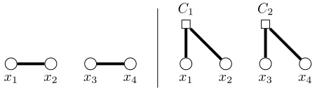
x1 x2 x3 x4 x1 x2 x3 x4
C1 C2
Figure 1: The primal graph (left) and the incidence graph (right) of the IQP instance given in Example 1.
in IQP is to compute an optimal solution for Iif one ex-ists, and otherwise to decide whether there exists a feasible assignment.
We note that aside from the inequality representation in-troduced above and used in other works (Lokshtanov 2015), IQP may equivalently be defined by havingFcontain only equalities and with explicit domains for individual variables. While using the former representation is more convenient for formalizing our contributions, none of the results pre-sented herein is sensitive to the specific representation used (changing the representation only changes our parameters by a multiplicative constant).
Finally, we will introduce two basic graph representations of IQP instances, which are also illustrated in Figure 1. Let I= (F, η)be an IQP instance. Theprimal graphofI, de-noted byP(I), is the undirected graph on var(I)having an edge between xandy if xandy occur together in a con-straint inF. Theincidence graphofI, denoted byH(I), is the bipartite graph with var(I)on one side,F on the other side, and there is an edge betweenx∈var(I)andA∈ F if and only ifxoccurs in the constraintA.
Parameterized Complexity
In parameterized algorithmics (Cygan et al. 2013; Nieder-meier 2006; Flum and Grohe 2006; Downey and Fellows 2013) the running time of algorithms is studied with respect to a parameterk ∈Nand input sizen. The basic idea is to
find a parameter that describes the structure of the instance such that the combinatorial explosion can be confined to this parameter. In this respect, the most favorable complex-ity class isFPT(fixed-parameter tractable) which contains all problems that can be decided by an algorithm running in timef(k)·nO(1), wheref is a computable function.
Al-gorithms with this running time are calledfixed-parameter algorithms.
One of the few (fixed-parameter) tractability results on IQP is due to Lokshtanov (2015) and can be viewed as an analogue to Lenstra’s classical result for Integer Linear Programming (Lenstra, Jr. 1983), but with additional condi-tions.
Proposition 2. An IQP instance I with ℓ = maxx∈var(I)coef(x) and k = max(|var(I)|, ℓ) can be solved in timeΛ(k,I) =f(k)·IO(1).
Structural Parameters
Here, we give an overview of the graph parameters that will be used in this paper. Atree-decomposition T of a graph
G = (V, E)is a pair(T, χ), where T is a tree andχis a function that assigns each tree nodet a set χ(t) ⊆ V of vertices such that the following conditions hold: (1) for ev-ery edge {u, v} ∈ E(G) there is a tree node t such that
u, v ∈ χ(t)and (2) for every vertexv ∈ V(G), the set of tree nodestwithv∈χ(t)forms a non-empty subtree ofT. The setχ(t)is also called the bag associated with the tree nodet. Thewidthof a tree-decomposition(T, χ)is the size of a largest bag minus1. A tree-decomposition of minimum width is calledoptimal. Thetreewidthof a graphGis the width of an optimal tree-decomposition ofG.
For presenting our dynamic programming algorithms, it is convenient to consider tree-decompositions in a normal form; such decompositions are callednice(Kloks 1994). A tree-decomposition (T, χ)of Gis niceifT is rooted at a node r withχ(r) = ∅ and each node ofT is one of the following four types:
1. aleaf node: a nodethaving no children and|χ(t)|= 1; 2. ajoin node: a nodethaving exactly two childrent1, t2,
andχ(t) =χ(t1) =χ(t2);
3. anintroduce node: a nodethaving exactly one childt′, andχ(t) =χ(t′)∪ {v}for a vertexvofG;
4. aforget node: a nodethaving exactly one childt′, and
χ(t) =χ(t′)\ {v}for a vertexvofG.
Fort∈ V(T)we denote byTtthe subtree ofT rooted att and writeχ(Tt)for the set⋃t′∈V(T
t)χ(t
′).
Proposition 3(Kloks 1994; Bodlaender 1996). It is possible to compute an optimal (nice) tree-decomposition of an n -vertex graphGwith treewidthkin timekO(k3)
n.
Our second parameter is called treedepth—a structural pa-rameter closely related to treewidth (Neˇsetˇril and Ossona de Mendez 2012). A useful way of thinking about graphs of bounded treedepth is that they are graphs of bounded treewidth with no long paths.
Since we will only need to directly work with treedepth in a single, technical lemma (notably Lemma 7), we refer to the book of Neˇsetˇil and de Mendez (2012) for the formal definition of the parameter.
IQP Lower Bounds
A simple reduction from SUBSETSUMgiven in (Murty and Kabadi 1987, Example 2) shows that IQP remainsNP-hard even if all variables are binary and the instance has only box constraints. We strengthen this result to instances with max-imum coefficient one. The starting point of our reduction is the well-knownNP-complete INDEPENDENTSETproblem.
Theorem 4. IQPisNP-hard even on instances with binary domain, maximum coefficient one, and where all constraints are box constraints.
Proof Sketch. Let(G, k)be an instance of INDEPENDENT SET. We construct an instanceIof IQP as follows: We set
var(I) = {xv | v ∈ V(G)}, F contains only box con-straints restricting the domain of each variable to{0,1}, and we setη= (∑
v∈V(G)xv)−(∑{u,v}∈E(G)xuxv). To com-plete the proof, it suffices to show thatGhas an independent set of size at leastkif and only if there is a solutionαforI withη(α)≥k.
Since our reduction preserves the size/value of a solution, it also can be used to carry over the known inapproxima-bility results for INDEPENDENTSET(H˚astad 1996) to IQP. Namely, we obtain that IQP cannot be approximated within a factor of|var(I)|1−ϵ, forϵ >0, unlessNP⊆ZPP.
Bounded Coefficients
In this section we study the setting where the input instances have bounded coefficients. Recently, Kouteck´y, Levin, and Onn (2018) showed that ILP is fixed parameter tractable pa-rameterized by the treedepth of the primal graph and the maximum left-hand side coefficient occurring in F. The lower bound result from the previous section shows that we cannot hope to obtain the same result for IQP unless we add additional restrictions on the objective function η. As our first and introductory result, we show that IQP is fixed pa-rameter tractable if we papa-rameterize by the maximum coef-ficient, the treedepth of the primal graph, and|var(η)|.
In the following letI= (F, η)be an IQP instance, td(I)
the treedepth ofP(I), andℓ(I)the maximum coefficient of I. We will now state our main result for this section.
Theorem 5. IQP is fixed-parameter tractable parameter-ized byℓ(I),td(I), and|var(η)|.
Before we proceed to the proof of above theorem, let us first argue its tightness. As mentioned previously, Theorem 4 shows that dropping|var(η)|from the parameterization re-sults in the problem becomingNP-hard even when the re-maining two parameters are bounded by a constant. The fol-lowing two known results then similarly rule out the possi-bility of dropping (or, in the case of treedepth, weakening) any of the other two parameters; note that ILP-feasibility is precisely IQP withη= 0.
Theorem 6(Ganian and Ordyniak 2018, Theorem 12 and 13). ILP-feasibility isNP-hard even for instances:
• with primal graphs of constant treedepth,
• with maximum coefficient one and primal graphs of treewidth at most two.
The proof of Theorem 5 uses the same strategy as the proof of an analogous theorem for ILP given by Ganian and Ordyniak (2018, Theorem 6). In particular, the algorithm for ILP can be divided into three steps:
(1) Compute an optimal treedepth decomposition ofP(I), (2) Using a bottom-up pruning procedure, the original ILP
instance is transformed into an equivalent ILP instance whose number of variables is bounded by a function of the parameters, and
Step (1) remains the same also in our proof of Theorem 5. In order to perform Step (2), we will obtain a more refined version of (Ganian and Ordyniak 2018, Lemma 11), which will then form the main tool for our pruning procedure.
Lemma 7. There exist computable functions f, g and an algorithm that takes as input I = (F, η) and an optimal treedepth decomposition of P(I), runs in time
O(f(ℓ(I),td(I),|var(η)|)· |I|)and outputs an IQP instance
I′ containing at most g(ℓ(I),td(I),|var(η)|)variables and whose maximum coefficient is no larger than the maximum coefficient ofIwith the following property: there exists a so-lutionαofIof valuewif and only if there exists a solution
α′ofI′of valuew. Moreover,αcan be computed fromα′in linear time.
Proof Sketch. The proof is very similar to the proof of Lemma 11 in (Ganian and Ordyniak 2018). The main dif-ference is due to a different definition of the primal graph in the cited proof, which additionally contains a clique on all variables contained in the objective function. It can be shown that adding a clique on all variables contained in the objective function only increases the treedepth by at most |var(η)|. After that, the remainder of the proof is virtually identical.
There are two main differences in the formulation of the above lemma compared to Lemma 11 in (Ganian and Or-dyniak 2018): (1) Both the running-time and the size of the reduced instance are given in terms of our parametersℓ(I), td(I), and|var(I)|and (2) we state explicitly that the coef-ficients of the pruned instance are no larger than the coeffi-cients in the original instance. The latter point is critical for our next Step (3), since we are required to use Proposition 2 instead of Lenstra’s algorithm in order to solve the instance obtained from Lemma 7.
Proof Sketch of Theorem 5. The algorithm proceeds as fol-lows. First, we compute a treedepth decomposition of
P(I) (Neˇsetˇril and de Mendez 2012). Second, we invoke Lemma 7 to obtain an equivalent instanceI′with only a few variables. Finally, we use Proposition 2 to solveI′.
We remark that due to the employed techniques, the running-time of the algorithm arising from Theorem 5 has a non-elementary dependency on the parameters. Hence, the result should be viewed primarily as a classification result.
Bounded Domain
It is known that ILP parameterized by the treewidth of the primal graph as well as the maximum absolute domain value of any variable is fixed-parameter tractable (Jansen and Kratsch 2015). Because of Theorem 4 this is not the case for IQP, i.e., IQP remainsNP-hard even when all vari-ables have a binary domain and the primal graph is edge-less. This is because having non-linear interactions between the variables in the optimization function implicitly allows the expression of linear constraints. To obtain tractability for IQP instances, it hence becomes necessary to also restrict the structure of the non-linear interactions between variables within the optimization function. To this end we propose the
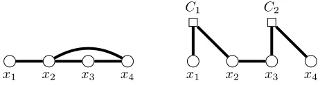
x1 x2 x3 x4
Figure 2: The mixed primal graph of the IQP instance given in Example 1.
mixed primal graph, denoted byPM(I), which extends the primal graph by adding an edge between any two distinct variablesxandythat occur together in a mixed term ofη
(see Figure 2 for an illustration of the mixed primal graph). Our main result for this section is establishing that the tractability for ILP using bounded domain and bounded treewidth of the primal graph carries over to IQP with the use of the mixed primal graph. In fact, we show tractability for the much more generalInteger Programming(IP) prob-lem, i.e., the generalization of IQP where both the objective function as well as the constraints are allowed to be arbitrary polynomials over the set of variables. Since known hardness results for ILP given in Theorem 6 carry over to IQP, it is es-sentially the case that the much more general IP exhibits the same complexity behavior on instances of boundedmixed primal treewidth as ILP on instances of bounded primal treewidth. Note, however, that the tractability results given in Theorem 5 for treedepth do not carry over to IP, since it is known that IP is undecidable even for instances with con-stantly many variables (K¨oppe 2012).
In the following letIbe an instance of IQP,T = (T, χ)
be a nice tree-decomposition ofPM(I)of widthω, and let
d= maxx∈var(I)dom(x).
Theorem 8. AnIPinstanceIcan be solved in timeO((2d+ 1)ω+2|I|), given that a nice tree-decomposition ofPM(I)of
widthωis provided with the input.
Before we proceed, let us formalize some additional nota-tion used in this secnota-tion. For a subsetV′of var(I), we denote byF[V′]the subset ofF containing all constraintsAsuch
that var(A)⊆V′. Letα:V′→Zbe a (partial) assignment,
x∈var(I), ands∈Z. We denote byαx→sthe assignment obtained fromαafter settingα(x) =s. Finally, we denote byI[V′]the subinstance ofIinduced byV′, i.e., the IP in-stance(F[V′], η[V′]).
We prove the theorem by giving a dynamic program-ming algorithm onT that computes the setR(t)of all valid records for every nodet ∈ V(T), where arecordis a pair
(α, o)consisting of an assignmentα:χ(t)→[−d, d]and an integero. A record(α, o)isvalidfortifois the maximum value forη(α′)over all feasible assignmentsα′:χ(Tt) →
[−d, d] for I[χ(Tt)] that agree with α on the variables in
χ(t). We show next how to compute the set of all valid records for each of the four node types ofT.
Lemma 9. R(t) can be computed from R(t′) in time
O(|R(t′)| ·d· |I|)for an introduce nodetofTwith childt′.
Proof Sketch. Let x be the variable introduced by t, i.e.,
χ(t) =χ(t′)∪ {x}. In this caseR(t)is the set of all pairs
(α, o+ (η[χ(t)]\η[χ(t′)])(α))with(α[χ(t′)], o)∈ R(t′)
R(t′) and every v ∈ [−d, d] and to evaluate the terms in(η[χ(t)]\ η[χ(t′)])for the assignment αx→v, which is
possible since all “new” constraints, i.e., the constraints in F(χ(t))\ F(χ(t′)), only contain variables inχ(t)and the same also holds for all terms inη(χ(t))\η(χ(t′)).
The computation ofR(t)for forget and join nodes follows similar lines as the proof of Lemma 9, and is trivial for leaf nodes. We summarize below.
Lemma 10. R(t) can be computed in time O((2d + 1)ω+1d|I|)for a leaf, forget, and join-nodet.
Proof Sketch for Theorem 8. The algorithm computes the set of all valid recordsR(t)for every nodet ofT using a bottom-up dynamic programming algorithm starting in the leaves ofT, until it computesR(r)for the root noder. It then outputsoifR(r) = {(∅, o)}and otherwise correctly returns thatIhas no optimal solution.
Theorem 8 together with Proposition 3 now imply that IP is fixed-parameter tractable parameterized by the maximum domain and the treewidth ofPM(I). Since IQP is a special case of IP, we obtain:
Corollary 11. IQPis fixed-parameter tractable parameter-ized by maximum domain and the treewidth ofPM(I).
Hybrid Restrictions
In this section, we turn our attention to instances where each variable is restricted in one of two possible ways: either the domain is bounded, or its maximum coefficient is bounded. Naturally, such instances are more general than those cov-ered in the first two settings, and hybrid restrictions may oc-cur naturally when modeling systems where variables repre-sent elements with different properties. Even though neither of the results and graph representations introduced up to this point can be used to obtain fixed-parameter algorithms for such instances, we will show that one can still exploit the treewidth of variable interactions to deal with such instances. Formally, the hybrid bound hyb(I) of an IQP instance Iis defined asmaxx∈var(I)min(dom(x),coef(x)). Observe
that every IQP instance with domain at most k or maxi-mum coefficient at mostk has a hybrid bound of at most
k, but the converse is not true. We note that IQP remains NP-hard even when both hyb(I)and the treewidth of the mixed primal graph are bounded by a constant; indeed, even ILP-feasibility remainsNP-hard when restricted to in-stances with a maximum coefficient of1and primal graphs of treewidth2(Ganian and Ordyniak 2018). The underlying reason for this is that variables with unbounded domain can, in some sense, carry long-distance interactions between vari-ables. We introduce thehybrid primal graphrepresentation in order to account for this and capture such interactions. For the purposes of this section, we will say that a variablexis
large-domainif dom(x)>hyb(I).
Definition 12. Thehybrid primal graphofI= (F, η)is the graphPH(I) = (V, E∪E′)where(V, E) =PM(I)andE′
is the set of all variable pairs that are connected by a path in
PM(I)whose internal vertices are large-domain variables.
x1 x2 x3 x4 x1 x2 x3 x4
C1 C2
Figure 3:Left:The hybrid primal graph of the IQP instance Igiven in Example 1. Observe that hyb(I) = 7andx3 is
the only large-domain variable.Right:The mixed incidence graph of the IQP instance given in Example 1.
We state our main result for this section below.
Theorem 13. IQPis fixed-parameter tractable parameter-ized byhyb(I)andtw(PH(I)).
Our first task on the way to proving Theorem 13 is to define a type of tree-decomposition that treats the large-domain variables (i.e., variables x such that dom(x) >
hyb(I)) in a certain way. To this end, we call a tree-decomposition ofPH(I)hybridif:
1. for each large-domain variablex, there exists a leaf node
tsuch thatx∈χ(t), and
2. every leaf nodethas a parentq(called theguard node) of degree 2 such thatχ(q)is obtained by removing all large-domain variables fromχ(t), and
3. all nodes other than guard and leaf nodes satisfy the con-ditions of nice tree-decompositions, i.e., are either forget, introduce or join nodes.
It is not difficult to show that any nice tree-decomposition of PH(I) can be transformed into a hybrid one in linear time—the core idea is to create new leaves that will con-tain the large-domain variables together with their neighbor-hood.
Our strategy for obtaining the fixed-parameter algorithm of Theorem 13 will now be the following. We will employ dynamic programming along the lines of Theorem 8; in par-ticular, at each nodetthat is neither a guard nor a leaf node, we will use the same records R(t) and apply Lemmas 9 and 10. Hence the crucial part will be to obtain the records
R(q)for each guard nodeq.
Lemma 14. Let (T, χ) be a hybrid width-k tree-decomposition of PH(I)and letq be a guard node inT.
Then it is possible to computeR(q)in time Λ(hyb(I),I)·
(2hyb(I) + 1)k· |I|O(1).
Proof Sketch. The procedure has two steps. First, we branch over all feasible assignments of the variables inχ(q). Sec-ond, for each such assignmentαwe apply Proposition 2 on the instance resulting by the application of α on I[χ(p)], wherepis the unique child ofq. It can be shown that this in-stance satisfies the conditions required by Proposition 2.
We can now proceed to a proof of the desired result.
is done, we proceed by dynamically computing the records for all other nodes inTin a leaves-to-root fashion by invok-ing Lemmas 9 and 10. Finally, we solve Iby reading the record at the root node r of T, in the same manner as in the proof of Theorem 8. The resulting runtime can be upper-bounded by|var(I)|times the runtime of Lemma 14.
Unary Coefficients and Unary Domain
In this section we generalize the polynomial-time algorithm for ILP with unary coefficients and unary domain using in-cidence treewidth (Ganian, Ordyniak, and Ramanujan 2017) to IQP. Again, because of our hardness result (Theorem 4), we will need additional restrictions on the variable depen-dencies expressed by mixed terms in the objective function. We therefore introduce themixed incidence graphof an IQP instanceI, denoted byHM(I), which is obtained from the incidence graph by adding edges between any two distinct variables occurring in mixed terms of the objective function (see Figure 3 for an illustration).In the following letI = (F, η)be an IQP instance and letT = (T, χ)be a nice tree-decomposition ofHM(I)of widthω. Similarly to the previous approach employed for ILP (Ganian, Ordyniak, and Ramanujan 2017), we will first show a slightly stronger result that will then imply tractabil-ity for unary domain and unary coefficients for constantω. LetΓbe the maximum absolute value of A(α)over every constraintA∈ Fand every feasible assignmentαforI. Theorem 15. IQP can be solved in time O(Γω+3ω3|I|) given that a nice tree decomposition ofHM(I)of widthωis
provided with the input.
As the algorithm uses dynamic programming on T, the overall structure of the algorithm is the same as for the algo-rithm presented in Theorem 8. We will hence only present the records together with the corresponding replacements of the lemmas required for showing the correctness for the four different node types ofT.
To distinguish between variables and constraints con-tained within the bags ofT, we use χvar(t)andχA(t)to denote the setsχ(t)∩var(I)andχ(t)∩ F, respectively. A
recordfor a nodet∈V(T)is a triple(α, γ, o), where: • α:χvar(t)→[−Γ,Γ],
• γ:χA(t)→[−Γ,Γ], and • ois a non-negative integer.
Note here that we use thatΓalso bounds the domain of every variable. We say that a record(α, γ, o)for a nodet∈V(T)
isvalidifois the maximum value ofη(α′)for any assign-mentα′:χvar(Tt)→[−Γ,Γ]satisfying:
R1 α′(x) =α(x)for every variablex∈χvar(t), R2 A(α′) =γ(A)for every constraintA∈χA(t).
We denote byR(t) the set of all valid records for t. The following lemma summarizes the computation for leaf, in-troduce, forget, and join nodes.
Lemma 16. R(t) can be computed in time
O(Γω+2ω2log Γ) for a leaf, introduce, forget, or join nodetofT.
Using Lemma 16, the proof of Theorem 15 now follows along the same lines as the proof of Theorem 8.
Note that together with Proposition 3, Theorem 15 implies polynomial-time tractability of IQP instances with bounded mixed incidence treewidth as long asΓcan be bounded by a polynomial of the input size. Namely, all tractability results considered in (Ganian, Ordyniak, and Ramanujan 2017) for ILP and bounded incidence treewidth carry over to IQP and boundedmixedincidence treewidth:
Corollary 17. IQPis solvable in polynomial-time for in-stances with bounded mixed incidence treewidth that addi-tionally satisfy either:
• unary domain and unary coefficients, or
• non-negativity and unary coefficients on the right-hand side of constraints.
An IQP instance isnon-negative if so is the domain of all variables as well as all coefficients occurring on the left-hand side of constraints.
Similarly, the hardness results given for ILP-feasibility by Ganian, Ordyniak and Ramanujan (2017) carry over to IQP, i.e., IQP isNP-hard for non-negative instances with binary domain and mixed incidence treewidth at most three as well as instances with maximum coefficient two and mixed inci-dence treewidth at most three.
Note, however, that we cannot (at least not directly) gen-eralize our tractability result for IQP for bounded mixed in-cidence treewidth to IP. Informally this is because even the mixed incidence treewidth does not take into account depen-dencies between variables that arise from mixed terms in the constraints.
Theorem 18. IP-feasibility is NP-hard even for instances with mixed incidence treewidth one, binary domain vari-ables, and maximum coefficient one.
Proof Sketch. The reduction is similar to our reduction from INDEPENDENT SETused in Theorem 4 only that this time we model the objective function as a constraint.
We note that it would be possible to generalize our algo-rithm given in Theorem 15 to IP, if we were to extend the mixed incidence graph by adding all edges between vari-ables that appear together in mixed terms of the constraints. Since IQP and not IP is the focus of this paper, we decided against providing the algorithm in its full generality.
Concluding Notes
Our results provide the first (and already surprisingly de-tailed) picture of the complexity of IQP w.r.t. natural struc-tural and syntactical restrictions. To our surprise, IQP be-haves very similar to the much simpler ILP once the role of the mixed terms in the optimization function is taken into account. Our results raise several interesting questions con-cerning the complexity of IQP and even ILP, and we high-light two such questions below:
2. What is the complexity of IQP (and ILP) parameterized by the treedepth of the mixed primal graph and hyb(I)?
The latter question is particularly interesting in light of the recently growing interest in multi-stage stochastic ILPs (Kouteck´y, Levin, and Onn 2018), whereas ILP in-stances with bounded primal treedepth and hyb(I)are sig-nificantly more general than multi-stage stochastic ILPs.
Acknowledgments.The authors wish to thank the reviewers for their insightful comments. Eduard Eiben was supported by Pareto-Optimal Parameterized Algorithms (ERC Starting Grant 715744) and by Parameterized Complexity for Practi-cal Computing (RCN Toppforsk Grant 274526). Robert Ga-nian acknowledges support from the FWF Austrian Science Fund (Project P31336:NFPC) and is also affiliated with FI MU, Brno, Czech Republic. Duˇsan Knop is partially sup-ported by DFG project MaMu (NI369/19) and is also affili-ated with Department of Theoretical Computer Science, FIT,
ˇ
CVUT, Prague, Czech Republic.
References
Aziz, H.; Gaspers, S.; Lee, E. J.; and Najeebullah, K. 2018. Defender stackelberg game with inverse geodesic length as utility metric. In Proc. AAMAS 2018, 694–702. Interna-tional Foundation for Autonomous Agents and Multiagent Systems.
Bodlaender, H. L. 1996. A linear-time algorithm for finding tree-decompositions of small treewidth. SIAM J. Comput.
25(6):1305–1317.
Crampton, J.; Gutin, G. Z.; Kouteck´y, M.; and Watrigant, R. 2017. Parameterized resiliency problems via integer linear programming. InProc. CIAC 2017, volume 10236 of Lec-ture Notes in Computer Science, 164–176.
Cygan, M.; Fomin, F. V.; Kowalik, L.; Lokshtanov, D.; Marx, D.; Pilipczuk, M.; Pilipczuk, M.; and Saurabh, S. 2013. Parameterized Algorithms. Texts in Computer Sci-ence. Springer.
Del Pia, A., and Weismantel, R. 2014. Integer quadratic programming in the plane. In Chekuri, C., ed.,Proc. SODA 2014, 840–846.
Del Pia, A.; Dey, S. S.; and Molinaro, M. 2017. Mixed-integer quadratic programming is in NP. Math. Program.
162(1-2):225–240.
Downey, R. G., and Fellows, M. R. 2013. Fundamentals of Parameterized Complexity. Texts in Computer Science. Springer.
Dvoˇr´ak, P.; Eiben, E.; Ganian, R.; Knop, D.; and Ordyniak, S. 2017. Solving integer linear programs with a small num-ber of global variables and constraints. In Sierra, C., ed.,
Proc. IJCAI 2017, 607–613. ijcai.org.
Eiben, E.; Ganian, R.; Knop, D.; and Ordyniak, S. 2018. Unary integer linear programming with structural restric-tions. InProc. IJCAI 2018, 1284–1290. ijcai.org.
Flum, J., and Grohe, M. 2006. Parameterized Complexity Theory, volume XIV ofTexts in Theoretical Computer Sci-ence. An EATCS Series. Berlin: Springer.
Ganian, R., and Ordyniak, S. 2018. The complexity land-scape of decompositional parameters for ilp.Artificial Intel-ligence257:61 – 71.
Ganian, R.; Ordyniak, S.; and Ramanujan, M. S. 2017. Go-ing beyond primal treewidth for (M)ILP. In SGo-ingh, S. P., and Markovitch, S., eds.,Proc. AAAI 2017, 815–821. AAAI Press.
H˚astad, J. 1996. Clique is hard to approximate within n1-epsilon. InProc. FOCS 1996, 627–636.
Iwashita, H.; Ohori, K.; Anai, H.; and Iwasaki, A. 2016. Simplifying urban network security games with cut-based graph contraction. In Proc. AAMAS 2016, AAMAS ’16, 205–213. International Foundation for Autonomous Agents and Multiagent Systems.
Jansen, B. M. P., and Kratsch, S. 2015. A structural approach to kernels for ILPs: Treewidth and total unimodularity. In
Proc. ESA 2015, volume 9294 ofLecture Notes in Computer Science, 779–791. Springer.
Kloks, T. 1994. Treewidth, Computations and Approxima-tions, volume 842 of Lecture Notes in Computer Science. Springer.
K¨oppe, M. 2012. On the complexity of nonlinear mixed-integer optimization. InMixed Integer Nonlinear Program-ming. Springer. 533–557.
Kouteck´y, M.; Levin, A.; and Onn, S. 2018. A Parameter-ized Strongly Polynomial Algorithm for Block Structured Integer Programs. In Chatzigiannakis, I.; Kaklamanis, C.; Marx, D.; and Sannella, D., eds.,Proc. ICALP 2018, volume 107 of LIPIcs, 85:1–85:14. Dagstuhl, Germany: Schloss Dagstuhl–Leibniz-Zentrum fuer Informatik.
Lenstra, Jr., H. W. 1983. Integer programming with a fixed number of variables. Math. Oper. Res.8(4):538–548. Lokshtanov, D. 2015. Parameterized integer quadratic programming: Variables and coefficients. CoRR
abs/1511.00310.
Murty, K. G., and Kabadi, S. N. 1987. Some np-complete problems in quadratic and nonlinear programming. Math. Program.39(2):117–129.
Neˇsetˇril, J., and de Mendez, P. O. 2012. Sparsity - Graphs, Structures, and Algorithms, volume 28 ofAlgorithms and combinatorics. Springer.
Neˇsetˇril, J., and Ossona de Mendez, P. 2012. Sparsity: Graphs, Structures, and Algorithms, volume 28 of Algo-rithms and Combinatorics. Springer.
Niedermeier, R. 2006. Invitation to Fixed-Parameter Algo-rithms, volume 31 ofOxford Lecture Series in Mathematics and its Applications. Oxford: Oxford University Press. Robertson, N., and Seymour, P. D. 1983. Graph minors. i. excluding a forest.J. Comb. Theory, Ser. B35(1):39–61. Shaloudegi, K.; Gy¨orgy, A.; Szepesv´ari, C.; and Xu, W. 2016. SDP relaxation with randomized rounding for energy disaggregation. InProc. NIPS 2016, 4979–4987.