The Thirty-Third AAAI Conference on Artificial Intelligence (AAAI-19)
N
E
VAE: A Deep Generative Model for Molecular Graphs
Bidisha Samanta
∗ IIT Kharagpur [email protected]Abir De
MPI-SWS [email protected]Gourhari Jana
IIT Kharagpur [email protected]Pratim Kumar Chattaraj
IIT KharagpurNiloy Ganguly
IIT Kharagpur [email protected]Manuel Gomez Rodriguez
MPI-SWSAbstract
Deep generative models have been praised for their ability to learn smooth latent representation of images, text, and au-dio, which can then be used to generate new, plausible data. However, current generative models are unable to work with molecular graphs due to their unique characteristics—their underlying structure is not Euclidean or grid-like, they re-main isomorphic under permutation of the nodes labels, and they come with a different number of nodes and edges. In this paper, we propose NeVAE, a novel variational autoencoder for molecular graphs, whose encoder and decoder are spe-cially designed to account for the above properties by means of several technical innovations. In addition, by using mask-ing, the decoder is able to guarantee a set of valid proper-ties in the generated molecules. Experiments reveal that our model can discover plausible, diverse and novel molecules more effectively than several state of the art methods. More-over, by utilizing Bayesian optimization over the continuous latent representation of molecules our model finds, we can also find molecules that maximize certain desirable proper-ties more effectively than alternatives.
Introduction
Drug design aims to identify (new) molecules with a set of specified properties, which in turn results in a therapeutic benefit to a group of patients. However, drug design is still a lengthy, expensive, difficult, and inefficient process with low rate of new therapeutic discovery (Paul et al. 2010), in which candidate molecules are produced through chemical syn-thesis or biological processes. In the context of computer-aided drug design (Merz, Ringe, and Reynolds 2010), there is a great interest in developing automated, machine learn-ing techniques to discover sizeable numbers of plausible, di-verse and novel candidate molecules in the vast (1023−1060) and unstructured molecular space (Polishchuk, Madzhidov, and Varnek 2013). In recent years, there has been a flurry of work devoted to developing deep generative models for au-tomatic molecule design (Dai et al. 2018; Kusner et al. 2017; G´omez-Bombarelli et al. 2016; Simonovsky and Komodakis 2018; Jin, Barzilay, and Jaakkola 2018), which has predom-inantly followed two strategies. The first strategy (Dai et al. 2018; Kusner et al. 2017; G´omez-Bombarelli et al. 2016)
Copyright c2019, Association for the Advancement of Artificial Intelligence (www.aaai.org). All rights reserved.
consists of representing molecules using a domain specific textual representation—SMILES strings—and then leverag-ing deep generative models for text generation for molecule design. Unfortunately, SMILE strings do not capture the structural similarity between molecules and, moreover, a molecule can have multiple SMILES representations. As a consequence, the generated molecules lack in terms of di-versity and validity, as shown in Tables 1–2 and Figure 3. The second strategy (Simonovsky and Komodakis 2018; Jin, Barzilay, and Jaakkola 2018) consists of representing molecules using molecular graphs, rather than SMILES rep-resentations, and then developing deep generative models for molecular graphs, in which atoms correspond to nodes and bonds correspond to edges. However, current generative models for molecular graphs share one or more of the fol-lowing limitations, which preclude them from realizing all their potential: (i) they can only generate (and be trained on) molecules with the same number of atoms while, in practice, molecules having similar properties often come with a dif-ferent number of atoms and bonds; (ii) they are not invariant to permutations of their node labels, however, graphs remain isomorphic under permutation of their node labels; (iii) their training procedure suffers from a quadratic complexity with respect to the number of nodes in the graph, which make it difficult to leverage a sizeable number of large molecules during training; and, (iv) they generate molecular graphs by combining a small set of moleculargraphlets(or subgraphs). The above shortcomings constrain the diversity of the gen-erated molecules, as shown in Table 1 and Figure 3.
In this paper, we develop NeVAE, a deep generative model for molecular graphs based on variational autoen-coders that overcomes the above shortcomings. To do so, it relies on several technical innovations, which distinguish us from previous work (Dai et al. 2018; Kusner et al. 2017; G´omez-Bombarelli et al. 2016; Simonovsky and Komodakis 2018; Jin, Barzilay, and Jaakkola 2018):
(i) Our probabilistic encoder learns to aggregate informa-tion (e.g., atom and bond features) from a different num-ber of hops away from a given atom and then map this aggregate information into a continuous latent space, as in inductive graph representation learning (Hamilton,
∗
Ying, and Leskovec 2017; Lei et al. 2017). However, in contrast with inductive graph representation learning, the aggregator functions are learned via variational inference so that the resulting aggregator functions are especially well suited to enable the probabilistic decoder to gen-erate new molecules rather than other downstream ma-chine learning tasks such as,e.g., link prediction. More-over, by using (symmetric) aggregator functions, it is in-variant to permutations of the node labels and can encode graphs with a variable number of atoms, as opposed to existing graph generative models, with a few the notable exception of those based on GCNs (Kipf and Welling 2016b).
(ii) Our probabilistic decoder jointly represents all edges as an unnormalized log probability vector (or ‘logit’), which then feeds a single multinomial edge distribution. Such scheme allows for an efficient inference algorithm with O(l) complexity, where l is the number of true edges in the molecules, which is also invariant to per-mutations of the node labels. In contrast, previous work typically models the presence and absence of each po-tential edge using a Bernoulli distribution and this leads to inference algorithms withO(n2)complexity, wheren
is the number of nodes, which are not permutation in-variant.
(iii) Our probabilistic decoder is able to guarantee a set of lo-cal structural and functional properties in the generated graphs by using amask in the edge distribution defini-tion, which can prevent the generation of certain undesir-ableedges during the decoding process. While masking have been increasingly used to account for prior (expert) knowledge in generative models (G´omez-Bombarelli et al. 2016; Kusner et al. 2017) based on SMILES, their use in generative models for molecular graphs has been lacking.
We evaluate our model using molecules from two publicly available datasets, ZINC (Irwin et al. 2012) and QM9 (Ra-makrishnan et al. 2014), and show that our model beats the state of the art in terms of several relevant quality metrics,
i.e., validity, novelty and uniqueness.
We also observe that the resulting latent space represen-tation of molecules exhibit powerful semantics—we can smoothly interpolate between molecules—and generaliza-tion ability—we can generate (valid) molecules that are larger than any of the molecules in the datasets. Finally, by utilizing Bayesian optimization over the latent representa-tion, we can also identify molecules that maximize certain desirable properties more effectively than alternatives. We are releasing an open source implementation of our model in Tensorflow.1
Background on Variational Autoencoders
Variational autoencoders (Kingma and Welling 2013; Rezende, Mohamed, and Wierstra 2014) are characterized by a probabilistic generative modelpθ(x|z)of the observed variablesx ∈ RN given the latent vari-ables z ∈ RM, a prior distribution over the latent
vari-1
https://github.com/Networks-Learning/nevae
ablesp(z)and an approximate probabilistic inference model
qφ(z|x). In this characterization, pθ and qφ are arbitrary distributions parametrized by two (deep) neural networksθ
andφand one can think of the generative model as a prob-abilistic decoder, which decodes latent variables into ob-served variables, and the inference model as a probabilistic
encoder, whichencodesobserved variables into latent vari-ables.
Ideally, if we use the maximum likelihood principle to train a variational autoencoder, we should optimize the marginal log-likelihood of the observed data, i.e.,
ED[logpθ(x)], wherepD is the data distribution.
Unfortu-nately, computing logpθ(x)requires marginalization with respect to the latent variable z, which is typically in-tractable. Therefore, one resorts to maximizing a variational lower bound or evidence lower bound (ELBO) of the log-likelihood of the observed data,i.e.,
max θ maxφ ED
h
−KL(qφ(z|x)||p(z)) +Eqφ(z|x)logpθ(x|z)
i
.
Finally, note that the quality of this variational lower bound depends on the expressive ability of the approximate infer-ence modelqφ(z|x), which is typically assumed to be a nor-mal distribution whose mean and variance are parametrized by a neural networkφwith the observed dataxas an input.
NeVAE: A Variational Autoencoder
for Molecular Graphs
In this section, we first give a high-level overview of the de-sign of NeVAE, our variational autoencoder for molecular graphs, starting from the data it is designed for. Then, we describe more depth the key technical aspects of its in-dividual components. Finally, we elaborate on the training procedure, scalability and implementation details.
High-level overview.We observe a collection ofN molec-ular graphs {Gi = (Vi,Ei)}i∈[N], where Vi andEi denote
the corresponding set of nodes (atoms) and edges (bonds), respectively, and this collection may contain graphs with a different number of nodes and edges. Moreover, for each molecular graph G = (V,E), we also observe a set of node features F = {fu}u∈V and edge weights Y =
{yuv}(u,v)∈E. More specifically, the node features fu are
one-hot representations of the type of the atoms (i.e.,C,H,
N orO), and the edge weightyuv are the bond types (i.e., single, double, triple). Our goal is then to design a varia-tional autoencoder for molecular graphs that, once trained on this collection of graphs, has the ability of creating new plau-sible molecular graphs, including node features and edge weights. In doing so, it will also provide a latent representa-tion of any graph in the collecrepresenta-tion (or elsewhere) with mean-ingful semantics.
Following the above background on variational autoen-coders, we characterize NeVAE by means of:
—Prior: p(z1, . . . ,zn),where|V|=|F |=n∼Poisson(λn)
—Inference model (encoder):qφ(z1, . . . ,zn|V,E,F,Y)
—Generative model (decoder): pθ(E,F,Y|z1, . . . ,zn)
W1 W1
W1 W2W2W2 WWW3..K3..K3..K
ccc1(1, .., K), .., ccc|V|(1, .., K)
c1 c1 c1(K)
c2 c2 c2(K)
ccc|V|−1(K)
ccc|V|(K)
cccu(1, .., K)
cccv(1, .., K)
cccw(1, .., K) φ
φφenc(ccc∗(1, .., K)) µ µ µ1, .., µµµ|V| σ σ σ1, .., σσσ|V| Wh, bh
Wµ, bµ Wσ, bσ
G,F,Y
u u
v
v
w
w
cccv(j)→cccv(j+ 1)
zzzu
zzzv
zzzw
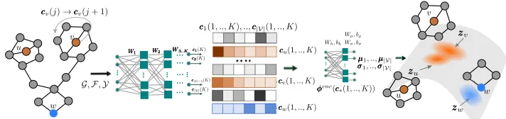
Figure 1: The encoder of our variational autoencoder for molecular graphs. From left to right, given a molecular graphGwith a set of node features F and edge weightsY, the encoder aggregates information from a different number of hopsj ≤ K
away for each nodev∈ Ginto an embedding vectorcv(j). These embeddings are fed into a differentiable functionφencwhich
parameterizes the posterior distributionqφ, from where the latent representation of each node in the input graph are sampled from.
a consequence, both the latent representation as well as the graph can vary in size. Next, we formally define the func-tional form of the inference model, the generative model, and the prior.
Inference model (probabilistic encoder). Given a graph G = (V,E)with node featuresFand edge weightsY, our inference modelqφdefines a probabilistic encoding for each node in the graph by aggregating information from differ-ent distances. More formally, for each nodeu, the inference model is defined as follows:
qφ(zu|V,E,F,Y)∼ N(µu,diag(σu)) (1)
where zu is the latent variable associated to node u,
[µu,diag(σu)] = φenc(cu(1), . . . ,cu(K)), andcu(k)
ag-gregates information fromkhops away fromu,i.e.,
cu(k) =
r(Wkfu) ifk= 1
r WkfuΛ ∪v∈N(u)yuvg(cv(k−1) ifk >1.
(2)
In the above,Wkare trainable weight matrices, which
prop-agate information between different search depths,Λ(.)is a (possibly nonlinear) symmetric aggregator function in its arguments,g(·)andr(·)are (possibly nonlinear) differen-tiable functions, φenc is a neural network, and
denotes pairwise product. Figure 1 describes our encoder architec-ture.
The above node embeddings, defined by Eq. 2, are very similar to the ones used in several graph representation learning algorithms such as GraphSAGE (Hamilton, Ying, and Leskovec 2017), column networks (Pham et al. 2017), and GCNs (Kipf and Welling 2016a), the main difference with our work is the way we will train the weight matrices
Wk. Here, we will use variational inference so that the
re-sulting embeddings are especially well suited to enable our probabilistic decoder to generate new, plausible molecular graphs. In contrast, the above algorithms use non variational approaches to compute general purpose embeddings to feed downstream machine learning tasks.
The following proposition highlights several desirable theoretical properties of our probabilistic encoder (details in arxiv version),2 which distinguishes our design from most existing generative models of graphs (Jin, Barzilay, and Jaakkola 2018; Simonovsky and Komodakis 2018):
2
https://arxiv.org/abs/1802.05283
Proposition 1 The probabilistic encoder defined by Eqs. 1 and 2 has the following properties:
(i) For each nodeu, its corresponding embedding cu(k)is invariant to permutations of the node labels of its neigh-bors.
(ii) The weight matricesW1, . . . ,Wk do not depend on the
number of nodes and edges in the graph and thus a sin-gle encoder allows for graphs with a variable number of nodes and edges.
Generative model (probabilistic decoder).Given a set of ofnnodes with latent variablesZ ={zu}u∈[n], our
gener-ative modelpθis defined as follows:
pθ(E,Y,F|Z) =pθ(F|Z)pθ(E,Y|Z), (3)
with
pθ(F |Z) = Y
u∈V
pθ(fu|Z),
pθ(E,Y|Z) =pθ(l
Z). pθ(E,Y|Z, l),
pθ(E,Y|Z, l) = Y
k∈[l]
pθ(ek|Ek−1,F,Z)pθ(yukvk|Yk−1,F,Z),
where the ordering for the edge and edge weights is in-dependent of node labels and hence permutation invariant,
ek andyukvk denote thek-th edge and edge weight under
the chosen order, andEk−1 ={e1, . . . , ek−1}andYk−1 =
{yu1v1, . . . , yuk−1vk−1}denote thek−1previously
gener-ated edges and edge weights respectively.
Moreover, the model characterizes the conditional proba-bilities in the above formulation as follows. For each node, it represents all potential node feature values fu = q as
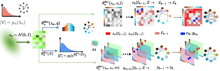
Figure 2: The decoder of our variational autoencoder for molecular graphs. From left to right, the decoder first samples the number of nodesn=|V|from a Poisson distributionpn(λn)and it samples a latent vectorzuper nodeu∈ VfromN(0,I). Then, for each nodeu, it represents all potential node feature values as an unnormalized log probability vector (or ‘logits’), where each entry is given by a nonlinearityθdec
γ of the corresponding latent representationzu, feeds this logit into a softmax
distribution and samples the node features. Next, it feeds all latent vectorsZinto a nonlinear log intensity functionθdecβ (Z)
which is used to sample the number of edges. Thereafter, on the top row, it constructs a logit for all potential edges(u, v), where each entry is given by a nonlinearityθdec
α of the corresponding latent representations(zu,zv). Then, it samples the edges one
by one from a soft max distribution depending on the logit and a maskxe(Ek−1), which gets updated every time it samples a
new edgeek. On the bottom row, it constructs a logit per edge(u, v)for all potential edge weight valuesm, where each entry is given by a nonlinearityθdec
ξ of the latent representations of the edge and edge weight value(zu,zv, m). Then, every time it
samples an edge, it samples the edge weight value from a soft max distribution depending on the corresponding logit and mask
xm(u, v), which gets updated every time it samples a newyukvk.
it prevents the generation of certainundesirableedges and edges weights, allowing for the generated graph to fulfill a set of predefined local structural and functional properties.
More formally, the distributions of each node feature, the number of edges, each edge and edge weight are given by:
pθ(fu=q|Z) =
eθγdec(zu,q)
P q0eθ
dec
γ (zu,q0), pθ(l
Z) =pl(eθ
dec
β (Z)),
pθ(e= (u, v)|Ek−1,Z) =
xeeθ
dec
α (zu,zv)
P
e0=(u0,v0)∈E/
k−1xe0e θdec
α (zu0,zv0)
,
pθ(yuv=m|Yk−1,Z) =
xm(u, v)eθ
dec
ξ (zu,zv,m)
P
m06=mxm0(u, v)eθ
dec
ξ (zu,zv,m0)
,
wherepl denotes a Poisson distribution,xe is the binary mask for edgee andxm(u, v)is the binary mask for fea-ture edge valuem, andθdec
• are neural networks. Note that
the parameters of the neural networks do not depend on the number of nodes or edges in the molecular graph and the de-pendency of the binary masksxeandxm(u, v)on the node features and the previously generated edgesEk−1 and edge
weightsYk−1 is deterministic and domain dependent.
Fig-ure 2 summarizes our decoder architectFig-ure.
Note that, by using a softmax distribution, it is only nec-essary to account for the presence of an edge, not its ab-sence, and this, in combination with negative sampling, will allow for efficient training and decoding, as it will become clear later in this section. This is in contrast with previ-ous generative models for graphs (Kipf and Welling 2016b; Simonovsky and Komodakis 2018), which need to model both the presence and absence of each potential edge. More-over, we would like to acknowledge that, while masking may
be useful to account for prior (expert) knowledge, it may be costly to check for some local (or global) structural and functional properties on-the-fly.
Prior. Given a set ofn nodes with latent variables Z =
{zu}u∈[n],pz(Z)∼ N(0,I).
Training.Given a collection ofN molecular graphs{Gi =
(Vi,Ei)}i∈[N], each with ni nodes, a set of node features
Fi and set of edge weights Yi, we train our variational
autoencoder for graphs by maximizing the evidence lower bound (ELBO), as described in the previous section, plus the log-likelihood of the Poisson distributionpλn modeling
the number of nodes in each graph. Hence we aim to solve:
maximize
φ,θ,λn
1
N X
i∈[N]
Eqφ(Zi|Vi,Ei,Fi,Yi)logpθ(Ei,Yi,Fi|Zi)
−KL(qφ||pz) + logpλn(ni)
(4)
Note that, in the above objective, computation of
Eqφlogpθ(Ei,Yi,Fi|Zi) requires to specify an order of
edges present in the graph Gi. To determine this order,
we use breadth-first-traversals (BFS) with randomized tie breaking during the child-selection step. Such a tie break-ing method makes the edge order independent of all node labels except for the source node label. Therefore, to make it completely permutation invariant, for each graph, we sample the source nodes from an arbitrary distribu-tion. More formally, we replace logpθ(Ei,Yi,Fi|Zi)with
logEs∼ζ(Vi)pθ(Ei,Yi,Fi|Zi)for each graphGi, wheresis
the randomly sampled source node for the BFS, and ζ is the sampling distribution fors. Note that, the logarithm of a marginalized likelihood is difficult to compute. Fortunately, by using Jensen inequality, we can have a lower bound of the actual likelihood:
Therefore, to train our model, we maximize
1
N X
i∈[N]
Eqφ(Zi|Vi,Ei,Fi,Yi),s∼ζ(Vi)logpθ(Ei,Yi,Fi|Zi)
−KL(qφ||pz) + logpλn(ni)
, (5)
The following theorem points out the key property of our objective function (proven in arxiv version).3
Theorem 2 If the source distributionζdoes not depend on the node labels, then the parameters learned by maximizing the objective in Eq. 5 are invariant to the permutations of the node labels.
Scalability and implementation details. In terms of scalability, the major bottleneck is computing the gra-dient of the first term in Eq. 5 during training, rather than encoding and decoding graphs once the model is trained. More specifically, given a source node for a net-work without masks, an exact computation of the per edge partition function of the log-likelihood of the edges,
i.e.,P
e0=(u0,v0)∈E/
k−1exp(θ dec
α (zu0,zv0)), requiresO(|V|2)
computations, similarly as in most inference algorithms for existing generative models of graphs, and hence is costly to compute even for medium networks. Fortunately, in prac-tice, we can approximate such partition function using neg-ative sampling (Mikolov et al. 2013) which reduces the like-lihood computation toO(l), wherel=|E|is the number of (true) edges in the graph. Therefore, forSsamples of source nodes, the complexity becomesO(Sl). Here, note that most real-world graphs are sparse and thusl |V|2.
Experiments on Real Data
In this section, we first show that our model beats sev-eral state of the art machine learning models for molecule design (Dai et al. 2018; G´omez-Bombarelli et al. 2016; Kusner et al. 2017; Simonovsky and Komodakis 2018; Jin, Barzilay, and Jaakkola 2018; Liu et al. 2018) in terms of several relevant quality metrics,i.e.,validity,noveltyand
uniqueness. Then, by applying Bayesian optimization over the latent space of molecules provided by our encoder, we also show that our model can find a greater number of molecules that maximize certain desirable properties. Fi-nally we show that the continuous latent representations of molecules that our model finds are smooth.
Experimental setup. We sample∼10,000 drug-like com-mercially available molecules from the ZINC dataset (Ir-win et al. 2012) with E[n] = 44 atoms and ∼10,000
molecules from the QM9 dataset (Ramakrishnan et al. 2014; Ruddigkeit et al. 2012) with E[n] = 21 atoms. For each molecule, we construct a molecular graph, where nodes are the atoms, the node features are the type of the atoms
i.e.fu ∈ {C, H, N, O}, edges are the bonds between two
atoms, and the weight associated to an edge is the type of bonds (single, double or triple)4. Then, for each dataset, we train our variational autoencoder for molecular graphs us-ing batches comprised of molecules with the same number
3
https://arxiv.org/abs/1802.05283 4
We have not selected any molecule whose bond types are others than these three.
of nodes5. Finally, we sample 106 molecular graphs from
each of the (two) trained variational autoencoders using: (i) G ∼ pθ(G|Z), whereZ ∼ p(Z)and (ii)Z ∼pθ(Z|G=
GT), whereGT is a molecular graph from the correspond-ing (traincorrespond-ing) dataset. In the above procedure, we only use masking on the weight (i.e., type of bond) distributions both during training and sampling to ensure that the valence of the nodes at both ends are valid at all times,i.e.,xm(u, v) = I(m+nk(u)≤mmax(u)∧m+nk(v)≤mmax(v)), where
nk(u)is the current valence of nodeuandmmax(u)is the maximum valence of node u, which depends on its type
fu. Moreover, during sampling, if there is no valid weight
value for a sampled edge, we reject it. To assess to which extent masking helps, we also train and sample from our model without masking. Here, we would like to highlight that, while using masking during test does not lead to signif-icant increase in the time it takes to generate a graph, using masking during training does lead to an increase of5% in training time.
We compare the quality of the molecules generated by our trained models and the molecules generated by sev-eral state of the art competing methods: (i) GraphVAE (Si-monovsky and Komodakis 2018), (ii) GrammarVAE (Kus-ner et al. 2017), (iii) CVAE (G´omez-Bombarelli et al. 2016), (iv) SDVAE (Dai et al. 2018), (v) JTVAE (Jin, Barzilay, and Jaakkola 2018) and (vi) CGVAE (Liu et al. 2018). Among them, GraphVAE, JTVAE and CGVAE use molecular graphs, however, the rest of the methods use SMILES strings, a domain specific textual representation of molecules. We use the following evaluation metrics for per-formance comparison:
(i) Novelty: we use this metric to evaluate to which degree a method generates novel molecules, i.e., molecules which were not present in the (training) dataset, i.e.
Novelty = 1− |Cs∩ D|/|Cs|, where Cs is the set of
generated molecules which are chemically valid,Dis the training dataset, and Novelty∈[0,1].
(ii) Uniqueness: we use this metric to evaluate to what extent a method generates unique chemically valid molecules. We define, Uniqueness = |set(Cs)|/ns
where ns is the number of generated molecules and Unique∈[0,1].
(iii) Validity: we use this metric to evaluate to which de-gree a method generates chemically valid molecules6. That is, Validity = |Cs|/ns where ns is the
num-ber of generated molecules,Csis the set of generated
molecules which are chemically valid, and note that Validity∈[0,1].
Quality of the generated molecules.Tables 1–2 compare our trained models to the state of the art methods above in terms of novelty, uniqueness, and validity. For GraphVAE and CGVAE we report the results reported in the paper and, for SDVAE, since there is no public domain implementation
5
We batch graphs with respect to the number of nodes for efficiency reasons since, every time that the number of nodes changes, we need to change the size of the com-putational graph in Tensorflow.
6
Novelty
Dataset NeVAE NeVAE∗ GraphVAE GrammarVAE CVAE SDVAE JTVAE CGVAE
ZINC 1.000 1.000 - 1.000 0.980 1.000 0.999 1.000
QM9 1.000 1.000 0.661 1.000 0.902 - 1.000 0.943
Uniqueness
Dataset NeVAE NeVAE∗ GraphVAE GrammarVAE CVAE SDVAE JTVAE CGVAE
ZINC 0.999 0.588 - 0.273 0.021 1.000 0.991 0.998
QM9 0.998 0.676 0.305 0.197 0.031 - 0.371 0.986
Table 1: Novelty and Uniqueness of the molecules generated using NeVAE and all baselines. The sign∗indicates no masking. For both the datasets, we report Novelty (Uniqueness) over valid (106) sampled molecules.
Validity
Dataset Sampling type NeVAE NeVAE∗ GraphVAE GrammarVAE CVAE SDVAE JTVAE CGVAE
ZINC Z∼P(Z)
Z∼P(Z|GT)
1.000 1.000
0.590 0.580
0.135
-0.440 0.381
0.021 0.175
0.432
-1.000 1.000
1.000
-QM9 Z∼P(Z)
Z∼P(Z|GT)
0.999 0.999
0.682 0.660
0.458
-0.200 0.301
0.031 0.100
-0.997 0.965
1.000
-Table 2: Validity the molecules generated using NeVAE and all baselines. The sign∗indicates no masking. For both the datasets, we report the numbers over106sampled molecules.
of these methods at the time of writing, we have used the sampled molecules from the prior provided by the authors for the ZINC dataset. For CVAE, GrammarVAE and JTVAE, we run their public domain implementations in the same set of molecules that we used. We find that, in terms of novelty, both our trained models and all competing methods except for the GraphVAE, which assumes a fixed number of nodes, are able to (almost) always generate novel molecules. How-ever, we would also like to note that novelty is only defined over chemically valid molecules. Therefore, despite hav-ing (almost) perfect novelty scores, all baselines except JT-VAE generate significantly fewer novel molecules than our method. In terms of uniqueness, which is defined over the set of sampled molecules, we observe that all baseline meth-ods, except CGVAE (for ZINC and QM9) and JTVAE (for ZINC), perform very poorly in both datasets in comparison with NeVAE. In terms of validity, our trained model signif-icantly outperform four competing methods—GraphVAE, GrammarVAE, CVAE and SDVAE—even without the use of masking, and achieve a comparable performance to JT-VAE and CGJT-VAE. In contrast to our model, GrammarJT-VAE,
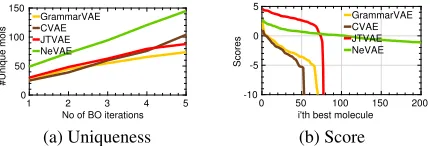
1 2 3 4 5
No of BO iterations 0
50 100 150
#Unique mols
GrammarVAE CVAE JTVAE NeVAE
(a) Uniqueness
0 50 100 150 200
i'th best molecule -10
-5 0 5
Scores
GrammarVAE CVAE JTVAE NeVAE
(b) Score
Figure 3: Property maximization using Bayesian optimiza-tion. Each plot shows the values ofy(m)in decreasing or-der for unique molecules. Panel (a) shows the variation of Uniqueness with the no. of BO iterations. Panel (b) shows the values ofy(m)sorted in the decreasing order.
Objective NeVAE GrammarVAE CVAE JTVAE
LL -1.45 -1.75 -2.29 -1.54
RMSE 1.23 1.38 1.80 1.25
Fraction ofvalidmolecules 1.00 0.77 0.53 1.00
Fraction ofuniquemolecules 0.58 0.29 0.41 0.32
Table 3: Property prediction performance (LL and RMSE) using Sparse Gaussian processes (SGPs) and property max-imization using Bayesian Optmax-imization (BO).
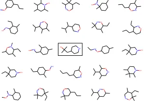
y(m) = 2.826(1st) y(m) = 2.477(2nd) y(m) = 2.299(3rd)
Figure 4: Best molecules found by Bayesian Optimization (BO) using our model.
CVAE and SDVAE use SMILES, a domain specific string based representation, and thus they may be constrained by its limited expressiveness. Among them, GrammarVAE and SDVAE achieve better performance by using a grammar to favor valid molecules. GraphVAE generates molecular graphs, as our model, however, its performance is inferior to our method because it assumes a fixed number of nodes, it samples edges independently from a Bernoulli distribution, and is not permutation invariant.
Bayesian optimization. Here, we leverage our model to discover novel molecules with desirable properties. Simi-larly as in previous work (G´omez-Bombarelli et al. 2016; Kusner et al. 2017; Jin, Barzilay, and Jaakkola 2018), we use Bayesian optimization (BO) to identify novel molecules
sam-(179.26, -3.03) (179.26, -3.99) (166.26, -4.05) (179.26, -4.86) (179.26, -4.76)
(179.26, -3.03) (179.26, -4.52) (179.26, -4.81) (179.26, -4.78) (179.26, -5.37)
(179.26, -3.03) (179.26, -4.78) (179.26, -4.81) (179.26, -4.40) (168.28, -4.09)
(179.26, -3.03) (179.26, -4.73) (165.23, -5.10) (165.26, -4.66) (166.26, -4.04)
(179.26, -3.03) (179.26, -4.90) (179.26, -4.62) (166.26, -4.38) (179.26, -5.23)
(a) ZINC dataset
(129.15, -4.51) (133.14, -4.27) (166.16, -3.77) (103.16, -3.73) (103.16, -3.22)
(129.15, -4.51) (129.15, -4.89) (112.17, -4.72) (112.17, -5.13) (112.17, -3.78)
(129.15, -4.51) (120.15, -3.82) (116.16, -4.77) (100.16, -4.17) (99.17, -2.75)
(129.15, -4.51) (112.17, -4.30) (112.17, -4.91) (116.16, -2.99) (120.14, -3.26)
(129.15, -4.51) (120.15, -3.82) (116.16, -4.42) (103.16, -4.21) (112.17, -4.48)
(b) QM9 Dataset
Figure 5: Molecules sampled using the probabilistic decoderG ∼pθ(G|Z), whereZ = {zi+aizi|zi ∈ Z0, ai ≥ 0}and
ai are given parameters. In each row, we use same molecule setai > 0for a single arbitrary nodei(denoted as•) and set
aj= 0, j6=ifor the remaining nodes. Under each molecule we report its molecular weight and synthetic accessibility score.
Figure 6: Molecules sampled using probabilistic decoder,
i.e. Gi ∼ pθ(G|Z), given the (sampled) latent
representa-tionZ of a given molecule G from the ZINC dataset. The sampled molecules are topologically similar to each other as well as the original.
ple3,000molecules from our ZINC dataset, which we split into training (90%) and test (10%) sets. Then, for our model and each competing model with public domain implemen-tations, we train a sparse Gaussian process (SGP) (Snelson and Ghahramani 2006) with the latent representations and
y(m)values of100inducing points sampled from the train-ing set. The SGPs allow us to make predictions for the prop-erty values of new molecules in the latent spaces. Then, we run5 iterations of batch Bayesian optimization (BO) using the expected improvement (EI) heuristic (Jones, Schonlau, and Welch 1998), with50(new) latent vectors (molecules) per iteration. Here, we compare the performance of all mod-els using several quality measures: (a) the predictive per-formance of the trained SGPs in terms of log-likelihood (LL) and root mean square error (RMSE) on the test set and (b) the average valueE[y(m)], fraction of valid molecules
and fraction ofgoodmolecules,i.e.,y(m) >0, among the molecules found using EI.
Table 3, Figure 3 and Figure 4 summarize the results. In terms of log-likelihood and RMSE, the SGP trained us-ing the latent representations provided by our model
outper-forms all baselines. In terms of the property valuesE[y(m)]
of the discovered molecules and fraction of valid and good molecules, BO under NeVAE also outperforms all baselines. Here, we would like to highlight that, while BO under JT-VAE is able to find a few molecules with larger property value than BO under NeVAE, it is unable to discover a size-able set of unique molecules with high property values.
Smooth latent space of molecules.In this section, we first demonstrate (qualitatively) that the latent space of molecules inferred by our model is smooth. Given a molecule, along with its associated graph G, node features F and edge weightsY, we first sample its latent representationZ using our probabilistic encoder,i.e.,Z ∼ qφ(Z|G,F,Y). Then, given this latent representation, we generate various molec-ular graphs by sampling from our probabilistic decoder,i.e., Gi ∼ pθ(G|Z). Figure 6 summarizes the results for one
molecule from ZINC dataset, which show that the sampled molecules are topologically similar to the given molecule.
Next, we show that our encoder, once trained, creates a latent space representation of molecules with powerful se-mantics. In particular, since each node in a molecule has a latent representation, we can make fine-grained changes to the structure of a molecule by perturbing the latent represen-tation of single nodes. To this aim, we proceed by first select-ing one molecule withnnodes from the ZINC dataset. Given its corresponding graph, node features and edge weights,G, F andY, we sample its latent representationZ0. Then, we
sample new molecular graphsG from the probabilistic de-coderG ∼pθ(G|Z), whereZ={zi+aizi|zi∈ Z0, ai≥
Conclusions
In this work, we have introduced a variational autoencoder for molecular graphs, that is permutation invariant of the nodes labels of the graphs they are trained with, and allow for graphs with different number of nodes and edges. More-over, the decoder is able to guarantee a set of local structural and functional properties in the generated graphs through masking. Finally, we have shown that our variational au-toencoder can also be used to discover valid and diverse molecules with certain desirable properties more effectively than several state of the art methods.
Our work also opens many interesting venues for future work. For eg. in the design of our variational autoencoder, we have assumed graphs to be static, however, it would be interesting to augment our design to dynamic graphs by,
e.g., incorporating a recurrent neural network. We have per-formed experiments on a single real-world application,e.g., automatic chemical design, however, it would be interesting to explore other applicationse.g. an end-to-end generative modeling of molecules with specified properties.
Acknowledgements. B. Samanta was supported by a Google India Ph.D. Fellowship and the “Learning Repre-sentations from Network Data” project sponsored by Intel. P. K. Chattaraj would like to thank DST, New Delhi for the J.C.Bose National Fellowship.
References
Dai, H.; Tian, Y.; Dai, B.; Skiena, S.; and Song, L. 2018. Syntax-directed variational autoencoder for structured data. InICLR.
G´omez-Bombarelli, R.; Duvenaud, D.; Hern´andez-Lobato, J. M.; Aguilera-Iparraguirre, J.; Hirzel, T. D.; Adams, R. P.; and Aspuru-Guzik, A. 2016. Automatic chemical design using a data-driven continuous representation of molecules.
arXiv preprint arXiv:1610.02415.
Hamilton, W.; Ying, R.; and Leskovec, J. 2017. Inductive representation learning on large graphs.NIPS.
Irwin, J. J.; Sterling, T.; Mysinger, M. M.; Bolstad, E. S.; and Coleman, R. G. 2012. Zinc: a free tool to discover chemistry for biology. Journal of chemical information and modeling
52(7):1757–1768.
Jin, W.; Barzilay, R.; and Jaakkola, T. 2018. Junction tree variational autoencoder for molecular graph generation.
arXiv preprint arXiv:1802.04364.
Jones, D. R.; Schonlau, M.; and Welch, W. J. 1998. Effi-cient global optimization of expensive black-box functions.
Journal of Global optimization13(4):455–492.
Kingma, D. P., and Welling, M. 2013. Auto-encoding vari-ational bayes. arXiv preprint arXiv:1312.6114.
Kipf, T. N., and Welling, M. 2016a. Semi-supervised clas-sification with graph convolutional networks.
Kipf, T. N., and Welling, M. 2016b. Variational graph auto-encoders.arXiv preprint arXiv:1611.07308.
Kusner, M. J.; Paige; Brooks; and Hern´andez-Lobato, J. M. 2017. Grammar variational autoencoder. arXiv preprint arXiv:1703.01925.
Lei, T.; Jin, W.; Barzilay, R.; and Jaakkola, T. 2017. Deriv-ing neural architectures from sequence and graph kernels.
ICML.
Liu, Q.; Allamanis, M.; Brockschmidt, M.; and Gaunt, A. L. 2018. Constrained graph variational autoencoders for molecule design. arXiv preprint arXiv:1805.09076. Merz, K. M.; Ringe, D.; and Reynolds, C. H. 2010. Drug design: structure-and ligand-based approaches. Cambridge University Press.
Mikolov, T.; Sutskever, I.; Chen, K.; Corrado, G. S.; and Dean, J. 2013. Distributed representations of words and phrases and their compositionality. InNIPS.
Paul, S. M.; Mytelka, D. S.; Dunwiddie, C. T.; Persinger, C. C.; Munos, B. H.; Lindborg, S. R.; and Schacht, A. L. 2010. How to improve r&d productivity: the pharmaceutical industry’s grand challenge. Nature reviews Drug discovery
9(3):203.
Pham, T.; Tran, T.; Phung, D. Q.; and Venkatesh, S. 2017. Column networks for collective classification. In Proceed-ings of the Thirty-First AAAI Conference on Artificial Intel-ligence, 2485–2491.
Polishchuk, P. G.; Madzhidov, T. I.; and Varnek, A. 2013. Estimation of the size of drug-like chemical space based on gdb-17 data. Journal of computer-aided molecular design
27(8):675–679.
Ramakrishnan, R.; Dral, P. O.; Rupp, M.; and Von Lilien-feld, O. A. 2014. Quantum chemistry structures and proper-ties of 134 kilo molecules. Scientific data1:140022. Rezende, D. J.; Mohamed, S.; and Wierstra, D. 2014. Stochastic backpropagation and approximate inference in deep generative models. arXiv preprint arXiv:1401.4082. Ruddigkeit, L.; Van Deursen, R.; Blum, L. C.; and Rey-mond, J.-L. 2012. Enumeration of 166 billion organic small molecules in the chemical universe database gdb-17. Jour-nal of chemical information and modeling 52(11):2864– 2875.
Simonovsky, M., and Komodakis, N. 2018. Graphvae: To-wards generation of small graphs using variational autoen-coders.arXiv preprint arXiv:1802.03480.