R E S E A R C H
Open Access
Sparse coding of the modulation spectrum for
noise-robust automatic speech recognition
Sara Ahmadi
1,2†, Seyed Mohammad Ahadi
1*, Bert Cranen
2†and Lou Boves
2†Abstract
The full modulation spectrum is a high-dimensional representation of one-dimensional audio signals. Most previous research in automatic speech recognition converted this very rich representation into the equivalent of a sequence of short-time power spectra, mainly to simplify the computation of the posterior probability that a frame of an unknown speech signal is related to a specific state. In this paper we use the raw output of a modulation spectrum analyser in combination with sparse coding as a means for obtaining state posterior probabilities. The modulation spectrum analyser uses 15 gammatone filters. The Hilbert envelope of the output of these filters is then processed by nine modulation frequency filters, with bandwidths up to 16 Hz. Experiments using the AURORA-2 task show that the novel approach is promising. We found that the representation of medium-term dynamics in the modulation
spectrum analyser must be improved. We also found that we should move towards sparse classification, by modifying the cost function in sparse coding such that the class(es) represented by the exemplars weigh in, in addition to the accuracy with which unknown observations are reconstructed. This creates two challenges: (1) developing a method for dictionary learning that takes the class occupancy of exemplars into account and (2) developing a method for learning a mapping from exemplar activations to state posterior probabilities that keeps the generalization to unseen conditions that is one of the strongest advantages of sparse coding.
Keywords: Sparse coding/compressive sensing; Sparse classification; Modulation spectrum; Noise robust automatic
speech recognition
1 Introduction
Nobody will seriously disagree with the statement that most of the information in acoustic signals is encoded in the way in which the signal properties change over time and that instantaneous characteristics, such as the shape or the envelope of the short-time spectrum, are less important - though surely not unimportant. The dynamic changes over time in the envelope of the short-time spec-trum are captured in the modulation specspec-trum [1-3]. This makes the modulation spectrum a fundamentally more informative representation of audio signals than a sequence of short-time spectra. Still, most approaches in speech technology, whether it is speech recognition, speech synthesis, speaker recognition, or speech cod-ing, seem to rely on impoverished representations of the
*Correspondence: [email protected] †Equal contributors
1Amirkabir University of Technology, Hafez 424, 15875-4413 Tehran, Iran Full list of author information is available at the end of the article
modulation spectrum in the form of a sequence of short-time spectra, possibly extended with explicit information about the dynamic changes in the form of delta and delta-delta coefficients. For speech (and audio) coding, the reliance on sequences of short-time spectra can be explained by the fact that many applications (first and foremost telephony) cannot tolerate delays in the order of 250 ms, while full use of modulation spectra might incur delays up to a second. What is more, coders can rely on the human auditory system to extract and utilize the dynamic changes that are still retained in the output of the coders. If coders are used in environments and appli-cations in which delay is not an issue (music recording, broadcast transmission), we do see a more elaborate use of information linked to modulation spectra [4-6]. Here too, the focus is on reducing bit rates by capitalizing on the properties of the human auditory system. We are not aware of approaches to speech synthesis - where delay is not an issue - that aim to harness advantages offered by
the modulation spectrum. Information about the tempo-ral dynamics of speech signal by means of shifted delta cepstra has proven beneficial for automatic language and speaker recognition [7].
In this paper we are concerned with the use of mod-ulation spectra for automatic speech recognition (ASR), specifically noise-robust speech recognition. In this appli-cation domain, we cannot rely on the intervention of the human auditory system. On the contrary, it is now nec-essary to automatically extract the information encoded in the modulation spectrum that humans would use to understand the message.
The seminal research by [1] showed that modulation frequencies >16 Hz contribute very little to speech intel-ligibility. In [8] it was shown that attenuating modulation frequencies <1 Hz does not affect intelligibility either. Very low modulation frequencies are related to station-ary channel characteristics or stationstation-ary noise, rather than to the dynamically changing speech signal carried by the channel. The upper limit of the band with linguistically relevant modulation frequencies is related to the maxi-mum speed with which the articulators can move. This insight gave rise to the introduction of RASTA filtering in [9] and [10]. RASTA filtering is best conceived of as a form of post-processing applied on the output of oth-erwise conventional representations of the speech signal derived from short-time spectra. This puts RASTA filter-ing in the same category as, for example, Mel-frequency spectra and Mel-frequency cepstral coefficients: engi-neering approaches designed to efficiently approximate representations manifested in psycho-acoustic experi-ments [11]. Subsequent developexperi-ments towards harnessing the modulation spectrum in ASR have followed pretty much the same path, characterized by some form of addi-tional processing applied to sequences of short-time spec-tral (or cepsspec-tral) features. Perhaps somewhat surprisingly, none of these developments have given rise to substan-tial improvements of recognition performance relative to other engineering tricks that do not take guidance from knowledge about the auditory system.
All existing ASR systems are characterized by an archi-tecture that consists of a front end and a back end. The back end always comes in the form of a state network, in which words are discrete units, made up of a directed graph of subword units (usually phones), each of which is in turn represented as a sequence of states. Recognizing an utterance amounts to searching the path in a finite-state machine that has the maximum likelihood, given an acoustic signal. The link between a continuous audio signal and the discrete state machine is established by converting the acoustic signal into a sequence of likeli-hoods that a short segment of the signal corresponds to one of the low-level states. The task of the front end is to convert the signal into a sequence of state likelihood
estimates, usually at a 100-Hz rate, which should be more than adequate to capture the fastest possible articulation movements.
Speech coding or speech synthesis with a 100-Hz frame rate using short-time spectra yields perfectly intelligible and natural-sounding results. Therefore, it was only natu-ral to assume that a sequence of short-time spectra at the same frame rate would be a good input representation for an ASR system. However, already in the early seventies, it was shown by Jean-Silvain Liénard [12] that it was nec-essary to augment the static spectrum representation by so-called delta and delta-delta coefficients that represent the speed and acceleration of the change of the spectral envelope over time and that were popularized by [13]. For reasonably clean speech, this approach appears to be adequate.
Under acoustically adverse conditions, the recognition performance of ASR systems degrades much more rapidly than human performance [14]. Convolutional noise can be effectively handled by RASTA-like processing. Distortions due to reverberation have a direct impact on the modula-tion spectrum, and they also cause substantial difficulties for human listeners [15,16]. Therefore, much research in noise-robust ASR has focused on speech recognition in additive noise. Speech recognition in noise basically must solve two problems simultaneously: (1) one needs to determine which acoustic properties of the signal belong to the target speech and which are due to the background noise (the source separation problem), and (2) those parts of the acoustic representations of the speech signal which are not entirely obscured by the noise must be pro-cessed to decode the linguistic message (speech decoding problem).
conversion most of the additional information carried by the modulation spectrum is lost.
In this paper we explore the use of a modulation spec-trum front end that is based on time-domain filtering that does not require collapsing the output to the equivalent of one-third octave filters, but which still makes it pos-sible to estimate the posterior probability of the states in a finite-state machine. In brief, we first filter the speech signal with 15 gammatone filters (roughly equivalent to one-third octave filters) and we process the Hilbert enve-lope of the output of the gammatone filters with nine modulation spectrum filters [19]. The 135-dimensional (135-D) output of this system can be sampled at any rate that is an integer fraction of the sampling frequency of the input speech signal. For the conversion of the 135-D output to posterior probability estimates of a set of states, we use the sparse coding (SC) approach proposed by [20]. Sparse coding is best conceived of as an exemplar-based approach [21] in which unknown inputs are coded as positive (weighted) sums of items in an exemplar dictionary.
We use the well-known AURORA-2 task [22] as the platform for developing our modulation spectrum approach to noise-robust ASR. We will use the ‘standard’ back end for this task, i.e. a Viterbi decoder that finds the best path in a lattice spanned by the 179 states that result from representing 11 digit words by 16 states each, plus 3 states for representing non-speech. We expect that the effect of the additive noise is limited to a subset of the 135 output channels of the modulation spectrum analyser.
The major goal of this paper is to introduce a novel approach to noise-robust ASR. The approach that we propose is novel in two respects: we use the ‘raw’ out-put of modulation frequency filters and we use Sparse Classification to derive state posterior probabilities from samples of the output of the modulation spectrum fil-ters. We deliberately use unadorned implementations of both the modulation spectrum analyser and the sparse coder, because we see a need for identifying what are the most important issues that are involved with a funda-mentally different approach to representing speech signals and with converting the representations to state poste-rior estimates. In doing so we are fully aware of the risk that - for the moment - we will end up with word error rates (WERs) that are well above what is considered state-of-the-art [23]. Understanding the issues that affect the performance of our system most will allow us to propose a road map towards our final goal that combines advanced insight in what it is that makes human speech recognition so very robust against noise with improved procedures for automatic noise-robust speech recognition.
Our approach combines two novelties,viz. the features
and the state posterior probability estimation. To make it possible to disentangle the contributions and implications
of the two novelties, we will also conduct experiments in which we use conventional multi-layered perceptrons (MLPs) to derive state posterior probability estimates from the outputs of the modulation spectrum analyser. In section 4, we will compare the sparse classification approach with the results obtained with the MLP for esti-mating state posterior probabilities. This will allow us to assess the advantages of the modulation spectrum anal-yser, as well as the contribution of the sparse classification approach.
2 Method
2.1 Sparse classification front end
The approach to noise-robust ASR that we propose in this paper was inspired by [20] and [24], which introduced
sparse classification(SCl) as a technique for estimating the posterior probabilities of the lowest-level states in an ASR system. The starting point of their approach was a repre-sentation of noisy speech signals as overlapping sequences of up to 30 speech frames that together cover up to 300 ms intervals of the signals. Individual frames were rep-resented as Mel-frequency energy spectra, because that representation conforms to the additivity requirement imposed by the sparse classification approach. SC is an exemplar-based approach. Handling clean speech requires the construction of an exemplar dictionary that contains stretches of speech signals of the same length as the (overlapping) stretches that must be coded. The exem-plars must be chosen such that they represent arbitrary utterances. For noisy speech a second exemplar dictionary must be created, which contains equally long exemplars of the additive noises. Speech is coded by finding a small number of speech and noise exemplars which, added together with positive weights, accurately approximate an interval of the original signal. The algorithms that find
the best exemplars and their weights are called solvers;
all solvers allow imposing a maximum on the number of exemplars that are returned with a weight >0 so that it is guaranteed that the result is sparse. Different families of solvers are available, but some require that all coefficients in the representations of the signals and the exemplars are non-negative numbers. Least angle regression [25],
implemented by means of a version of theLassosolver,
can operate with representations that contain positive and negative numbers.
by means of a forced alignment of the database from which the exemplars are selected with the states that cor-respond to a phonetic transcription. In actual practice, the state labels are obtained by means of a forced align-ment using a conventional hidden Markov model (HMM) recognizer.
The success of the SC approach in [20,24] for noise-robust speech recognition is attributed to the fact that the speech exemplars are characterized by peaks in the spec-tral energy that exhibit substantial continuity over time; the human articulatory system can only produce signals that contain few clear discontinuities (such as the release of stop consonants), while many noise types lack such con-tinuity. Therefore, it is reasonable to expect that the mod-ulation spectra of speech and noise are rather different, even if the short-time spectra may be very similar.
In this paper we use the modulation spectrum directly to exploit the continuity constraints imposed by the speech production system. Since the modulation spec-trum captures information about the continuity of the speech signal in the low-frequency bands, there is no need for a representation that stacks a large number of subsequent time frames. Therefore, our exemplar dictio-nary can be created by selecting individual frames of the modulation spectrum in a database of labelled speech. As in [20,24], we will convert the weights assigned to the exemplars when coding unknown speech signals into esti-mates of the probability that a frame in the unknown signal corresponds to one of the states.
In [20,24] the conversion of exemplar weights into state probabilities involved an averaging procedure. A frame in an unknown speech signal was included in as many solu-tions of the solver as there were frames in an exemplar. In each position of a sliding window, an unknown frame is associated with the states in the exemplars chosen in that position. While individual window positions return a small number of exemplars and therefore a small num-ber of possible states, the eventual set of state probabilities assigned to a frame is not very sparse. With the single-frame exemplars in the approach presented here, no such averaging is necessary or possible. The potential down-side of relying on a single set of exemplars to estimate state probabilities is that it may yield overly sparse state probability vectors.
2.2 Data
In order to provide a proof of concept that our ap-proach is viable, we used a part of the AURORA-2 database [22]. This database consists of speech recordings taken from the TIDIGITS corpus for which participants read sequences of digits (only using the words ‘zero’ to ‘nine’ and ‘oh’) with one up to seven digits per utter-ance. These recordings were then artificially noisified by adding different types of noise to the clean recordings at
different signal-to-noise ratios. In this paper we focus on
the results obtained for test set A, i.e. the test set that
is corrupted using the same noise types that occur in the multi-condition training set. We re-used a previously made state-level segmentation of the signals obtained by means of a forced alignment with a conventional HMM-based ASR system. These labels were also used to estimate the prior probabilities of the 179 states.
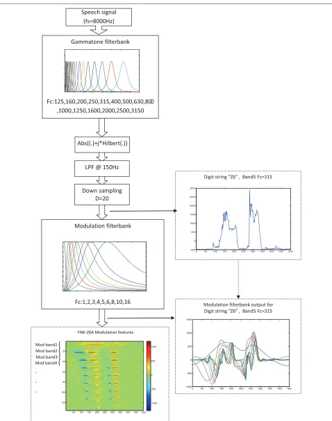
2.3 Feature extraction
The feature extraction process that we employ is illus-trated in Figure 1. First, the (noisy) speech signal
(sam-pling frequencyFs = 8 kHz) is analysed by agammatone
filterbank consisting of 15 band-pass filters with centre
frequencies (Fc) spaced at one-third octave. More
specifi-cally,Fc= 125, 160, 200, 250, 315, 400, 500, 630, 800, 1,000,
1,250, 1,600, 2,000, 2,500, and 3,150 Hz, respectively. The
amplitude response of annth-order gammatone filter with
centre frequencyFcis defined by
g(t)=a·tn−1·cos(2πFct+φ)·e−2πbt. (1)
With b = 1.0183 × (24.7+ Fc/9.265) and n = 4,
this yields band-pass filters with equivalent rectangular bandwidth equal to 1 [27]. Subsequently, the time enve-lope ei(t)of theith filter output,xi, is computed as the
magnitude of the analytic signal
ei(t)=
x2i + ˆx2i, (2)
withxˆi the Hilbert transform ofxi. We assume that the
time envelopes of the outputs of the gammatone filters are a sufficiently complete representation of the input speech signal. The frequency response of the gammatone filter-bank is shown in the upper part at the left-hand side of Figure 1.
The Hilbert envelopes were low-pass filtered with a
fifth-order Butterworth filter (cf. (3)) with cut-off
fre-quency at 150 Hz and down-sampled to 400 Hz. The down-sampled time envelopes from the 15 gammatone filters are fed into another filterbank consisting of nine modulation filters. This so-called modulation filterbank is similar to the EPSM-filterbank as presented by [28]. In our implementation of the modulation filterbank, we used one-third-order Butterworth low-pass filter with a cut-off frequency of 1 Hz, and eight band-pass filters with centre frequencies of 2, 3, 4, 5, 6, 8, 10, and 16 Hza.
The frequency response of annth-order low-pass filter
with gainaand cut-off frequencyFcis specified by [29]
H(f)= a
1.0+Ff
c
The complex-valued frequency response of a band-pass
modulation filter with gain a, centre frequency Fc and
quality factorQ=1 is specified by
H(f)= a
1.0+jQ.
f Fc −
Fc f
(4)
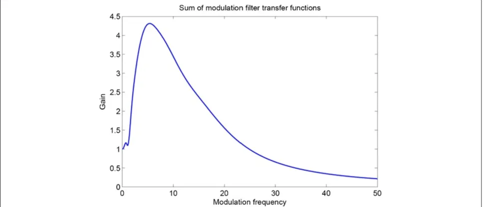
As an example, the upper panel at the right-hand side in Figure 1 shows the time envelope of the output of the gam-matone filter with centre frequency at 315 Hz for the digit sequence ‘zero six’. The frequency response of the com-plete filterbank, i.e. the sum of the responses of the nine individual filters, is shown in Figure 2. Due to the spac-ing of the centre frequency of the filters and the over-lap of their transfer functions, we effectively give more weight to the modulation frequencies that are dominant in speech [30].
The modulation frequency filterbank is implemented as a set of frequency domain filters. To obtain a frequency resolution of 0.1 Hz with the Hilbert envelopes sampled at 400 Hz, the calculations were based on Fourier transforms consisting of 4,001 frequency samples. For that purpose we computed the complex-valued frequency response of the filters at 4,001 frequency points. An example of the ensemble of waveforms that results from the combination of the gammatone and modulation filterbank analysis for the digit sequence ‘zero six’ is shown in the lower panel on the right-hand side of Figure 1. The amplitudes of the
9×15 = 135 signals as a function of time are shown in
the bottom panel at the left-hand side of Figure 1. The top band represents the lowest modulation frequencies (0 to 1 Hz) and the bottom band the highest (modulation filter
with centre frequencyFc=16 Hz).
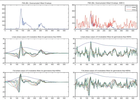
We experimented with two different implementations of the modulation frequency filterbank, one in which we kept the phase response of the filters and the other in which we ignored the phase response and only retained the magnitude of the transfer functions. The results are illustrated in Figure 3 for clean speech and for the 5-dB signal-to-noise ratio (SNR) condition. From the second and third rows in that figure, it can be inferred that the linear phase implementation renders sudden changes in the Hilbert envelope as synchronized events in all modu-lation bands, while the full-phase implementation appears to smear these changes over wider time intervals. The (visual) effect is especially apparent in the right column, where the noisy speech is depicted. However, prelimi-nary experiments indicated that the information captured in the ‘visually noisy’ full-phase representation could be harnessed by the recognition system: the full-phase imple-mentation yields a performance increase in the order of 20% at the lower SNR levels compared with the perfor-mance of the linear phase implementation. However, the linear phase implementation works slightly better in clean
and high SNR conditions (yielding ≈1% higher
accura-cies). This confirms the results of previous experiments in [31]. Therefore, all results in this paper are based on the full-phase implementation.
Another unsurprising observation that can be made from Figure 3 is that the non-negative Hilbert envelopes are turned into signals that have both positive and neg-ative amplitude values. This will limit the options in choosing a solver in the SC approach to computing state posterior probabilities.
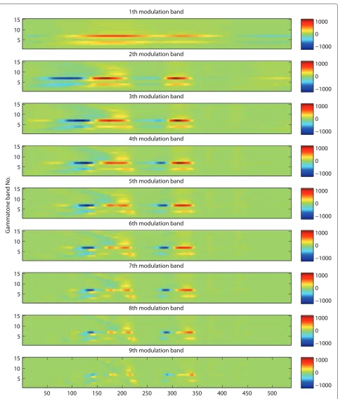
Figure 4 provides an extended view of the result of a modulation spectrum analysis of the utterance ‘zero six’.
Figure 3Full and linear phase features comparison.Top: spectrum envelope of 6th gammatone band for a sample utterance for clean (left) and 5-dB SNR (right). Middle: output of linear phase modulation filterbank. Bottom: output of full-phase modulation filterbank.
The nine heat map representations in the lower left-hand part of Figure 1 are re-drawn in such a way that it is pos-sible to see the similarities and differences between the modulation bands. The top panel in Figure 4 shows the output amplitude of the low-pass filter of the modulation filter bank. Subsequent panels show the amplitude of the outputs of the higher modulation band filters. It can be seen that overall, the amplitude decreases with increasing band number.
Speech and background noise tend to cover the same frequency regions in the short-time spectrum. Therefore, speech and noise will be mixed in the outputs of the 15 gammatone filters. The modulation filterbank decom-poses each of the 15 time envelopes into a set of nine time-domain signals that correspond to different mod-ulation frequencies. Generally speaking, the outputs of the lowest modulation frequencies are more associated with events demarcating syllable nuclei, while the higher modulation frequencies represent shorter-term events. We want to take advantage of the fact that it is unlikely that speech and noise sound sources with frequency
components in the same gammatone filter also happen to overlap completely in the modulation frequency domain. Stationary noise would not affect the output of the higher modulation frequency filters, while pulsatile noise should not affect the lowest modulation frequency filters. There-fore, we expect that many of the naturally occurring noise sources will show temporal variations at different rates than speech.
Although the modulation spectrum features capture short- and medium-time spectral dynamics, the informa-tion is encoded in a manner that might not be optimal for automatic pattern recognition purposes. Therefore, we decided to also create a feature set that encodes the temporal dynamics more explicitly. To that end we con-catenated 29 frames (at a rate of one frame per 2.5 ms),
corresponding to 29×2.5=72.5 ms; to keep the number
−1000 0 1000 9th modulation band
50 100 150 200 250 300 350 400 450 500
5 10 15
−1000 0 1000 8th modulation band
5 10 15
−1000 0 1000 7th modulation band
5 10 15
−1000 0 1000 6th modulation band
5 10 15
−1000 0 1000
Gammatone band No.
5th modulation band
5 10 15
−1000 0 1000 4th modulation band
5 10 15
−1000 0 1000 3th modulation band
5 10 15
−1000 0 1000 2th modulation band
5 10 15
−1000 0 1000 1th modulation band
5 10 15
Figure 4An extended view of the result of a modulation spectrum analysis of the utterance ‘zero six’.
learned using the exemplar dictionary (cf., section 2.4).
The dimension of the feature vectors was reduced the 135, the same number as with single-frame features. To be able to investigate the effect of the LDA transform, we
2.4 Composition of exemplar dictionary
To construct the speech exemplar dictionary, we first encoded the clean train set of AURORA-2 with the mod-ulation spectrum analysis system, using a frame rate of 400 Hz. Then, we quasi-randomly selected two frames from each utterance. To make sure that we had a rea-sonably uniform coverage of all states and both genders,
2×179 counters were used (one for each state of each
gen-der). The counters were initialized at 48. For each selected exemplar, the corresponding counter was decremented by 1. Exemplars of a gender-state combination were no longer added to the dictionary if the counter became zero. A simple implementation of this search strategy yielded a set of 17,148 exemplars, in which some states missed one or two exemplars. It appeared that 36 exemplars had
a Pearson correlation coefficient of>0.999 with at least
one other exemplar. Therefore, the effective size of the dictionary is 17,091.
We also encoded the four noises in the multi-condition training set of AURORA-2 with the modulation spectrum analysis system. From the output, we randomly selected 13,300 frames as noise exemplars, with an equal number of exemplars for the four noise types.
When using LDA-transformed concatenated features, a new equally large set of exemplars was created by selecting sequences of 29 consecutive frames, using the same proce-dures as for selecting single-frame exemplars. In a similar vein, 29-frame noise exemplars were selected that were reduced to 135-D features using the same transformation matrix as for the speech exemplars.
2.5 The sparse classification algorithm
The use of sparse classification requires that it must be possible to approximate an unknown observation with
a (positive) weighted sum of a number of exemplars. Since all operations in the modulation spectrum analysis system are linear and since the noisy signals were con-structed by simply adding clean speech and noise, we are confident that the modulation spectrum representation does not violate additivity to such an extent that SC is rendered impossible. The same argument holds for the LDA-transformed features. Since linear transformations do not violate additivity, we assume that the transformed exemplars can be used in the same way as the original ones.
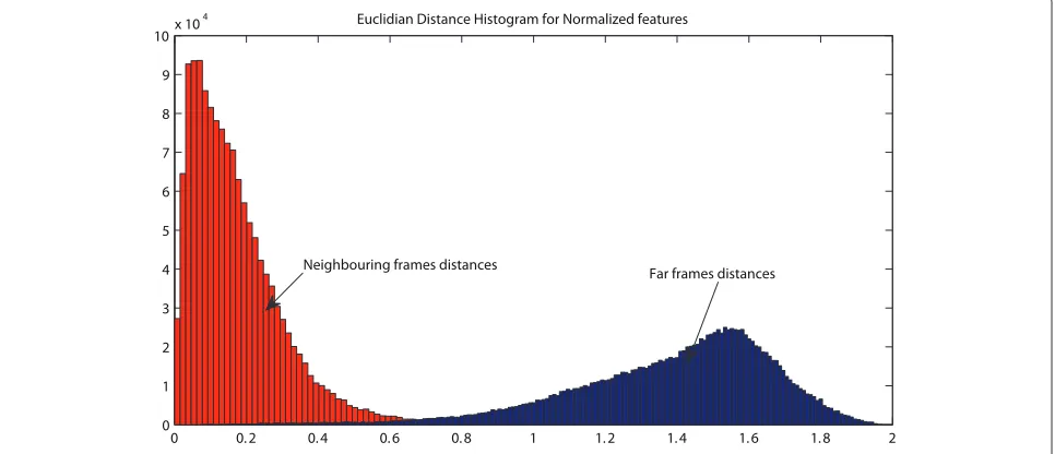
As can be seen in Figures 1 and 3, the output of the mod-ulation filters contains both positive and negative num-bers. Therefore, we need to use the Lasso procedure for solving the sparse coding problem, which can operate with positive and negative numbers [25]. We are not aware of other solvers that offer the same freedom. Lasso uses the Euclidean distance as the divergence measure to evaluate the similarity of vectors. This raises the question whether the Euclidean distance is a suitable measure for comparing modulation spectrum vectors. We verified this by com-puting the distributions of the Euclidean distance between neighbouring frames and frames taken at random time
distances of>20 frames in a set of 100 randomly selected
utterances. As can be seen from Figure 5, the distributions of the distances between neighbouring and distant frames hardly overlap. Therefore, we believe that it is safe to assume that the Euclidean distance measure is adequate.
Using the Euclidean distance in a straightforward man-ner implies that vector elements that have a large variance or large absolute values will dominate the result. Prelim-inary experiments showed that the modulation spectra suffer from this effect. It appeared that the difference
between /u/ in two and /i/ in three, which is mainly
represented by different energy levels in the 2,000-Hz
0 0. 2 0. 4 0. 6 0. 8 1 1. 2 1. 4 1. 6 1. 8 2
0 1 2 3 4 5 6 7 8 9 10x 10
4 Euclidian Distance Histogram for Normalized features
Neighbouring frames distances
Far frames distances
region, was often very small because of the absolute values of the output of the modulation filters in the gammatone filters with centre frequencies of 2,000 and 2,500 Hz which were very much smaller than the values in the gammatone filters with centre frequencies up to 400 Hz. This effect can be remedied by using a proper normalization of the vector elements. After some experiments, we decided to equalize the variance in the gammatone bands. For this purpose we first computed the variance in all 135 mod-ulation bands in the set of speech exemplars. Then, we averaged the variance over the nine modulation bands in each gammatone filter. The resulting averages were used to normalize the outputs of the modulation filters. The effect of this procedure on the representation of the out-put of the modulation filters is shown in Figure 6. This procedure reduced the number of /u/ - /i/ confusions by almost a factor of 3.
2.5.1 Obtaining state posterior estimates
The weights assigned to the exemplars by the Lasso solver must be converted to estimates of the probability that a frame corresponds to one of the 179 states. In the sparse
classification system of [20], weights of up to 30 window positions were averaged. In our SC system, we do not have a sliding window with heavy overlap between subsequent positions. We decided to use the weights of the exemplars that approximate individual frames to derive the state pos-terior probability estimates. In doing so, we simply added the weights of all exemplars corresponding to a given state. The average number of non-zero elements in the activa-tion vector varied between 15.1 for clean speech and 6.5
at−5-dB SNR. Therefore, we may face overly sparse and
potentially somewhat noisy state probability estimates. This is illustrated in Figure 7a for the digit sequence ‘3 6 7’ in the 5-dB SNR condition. The traces of state probability estimates are not continuous (do not traverse all 16 states of a word) and they include activations of other states, some of which are acoustically similar to the states that correspond to the digit sequence.
2.6 Recognition based on combinations of individual modulation bands
Substantial previous research has investigated the possi-bility to combat additive noise by fusing the outputs of a
Figure 7State probability traces for the digit sequence ‘3 6 7’ at 5-dB SNR.(a)Traces obtained by using the activation weights of the full modulation spectrum exemplars only. The Viterbi decoder returns the incorrect sequence ‘3 3 7’.(b)Traces obtained from fusing the probability estimates obtained with the full modulation spectrum and the probability estimates obtained from nine modulation bands (weights obtained with a genetic algorithm). The Viterbi decoder now returns the correct sequence ‘3 6 7’.
number of parallel recognizers, each operating on a
sepa-rate frequency band (cf., [32] for a comprehensive review).
The general idea underlying this approach is that additive noise will only affect some frequency bands so that other bands should suffer less. The same idea has also been pro-posed for different modulation bands [33]. In this paper we also explore the possibility that additive noise does not affect all modulation bands to the same extent. Therefore, we will compare recognition accuracies obtained when estimating state likelihoods using a single set of exem-plars represented by 135-D feature vectors and the fusion of the state likelihoods estimated from the 135-D sys-tem and nine sets of exemplars (one for each modulation band) represented as 15-D feature vectors (for the 15 gam-matone filters). The optimal weights for the nine sets of estimates will be obtained using a genetic algorithm with
a small set of held-out training utterances. Also, combin-ing state posterior probability estimates from ten decoders might help to make the resulting probability vectors less sparse.
2.7 State posteriors estimated by means of an MLP
In order to tease apart the contributions of the modu-lation frequency features and the sparse coding, we also conducted experiments in which we used a MLP for esti-mating the posterior probabilities of the 179 states in the AURORA-2 task. For this purpose we trained a number of networks by means of the QuickNet software pack-age [34]. We trained networks on clean data only, as well as on the full set of utterances in the multi-condition training set. Analogously to [35], we used 90% of the train-ing set, i.e. 7,596 utterances for traintrain-ing the MLP and the remaining 844 utterances for the cross-validation. To enable a fair comparison, we trained two networks, both operating on single frames. The first network used frames consisting of 135 features; the second network used ‘static’ modulation frequency features extended with delta and delta-delta features estimated over a time interval of 90 ms, making for 405 input features. The delta and delta-delta features were obtained by fitting a linear regression on the sequence of feature values that span the 90-ms intervals. Actually, the 90-ms interval corresponds to the time interval covered by the perceptual linear prediction (PLP) features used in [35]. There too, the static PLP features were extended by delta and delta-delta features,
making for 9×39=351 input nodes.
3 Results
The recognition accuracies obtained with the 135-D mod-ulation spectrum features are presented in the top part of Tables 1 and 2 for the SC-based system. The second and third rows of Table 2 show the results for the MLP-based system. Both tables also contain results obtained previ-ously with conventional Mel-spectrum or PLP features. Note that the results in Table 1 pertain to a single-noise condition of test set A (subway noise), while Table 2 shows the accuracies averaged over all four noise types in test set A. In experimenting with the AURORA-2 task, it is a pervasive finding that the results depend strongly on the word insertion penalty (WIP) that is used in the Viterbi back end. A WIP that yields the lowest WER in the clean condition invariably gives a very high WER in the noisiest conditions. In this paper we set aside a small development set, on which we searched the WIP that
gave the best results in the conditions with SNR≤ 5 dB;
Table 1 Accuracy for five systems on noise type 1 (subway noise) of test set A
Clean 20 dB 15 dB 10 dB 5 dB 0 dB −5 dB
Sys1 90.51 91.00 89.53 87.69 83.76 76.76 65.31
(single frame)
Sys2
(single frame) 89.19 89.62 87.57 83.54 76.51 62.57 36.91
(LDA transformed)
Sys3
(29 frames) 87.50 88.70 87.41 85.42 77.62 59.41 27.85
(LDA transformed)
Sys4 89.71 90.57 89.28 87.41 84.13 77.71 63.83
(9 bands - GA)
Sparse coding [24] 93.12 90.18 87.22 82.62 72.64 56.31 34.57
5-frame exemplars
Sparse coding [24] 93.21 91.86 91.53 89.62 87.47 80.01 61.61
30-frame exemplars
Sys1, 135-D vectors; Sys2, LDA-transformed 135-D vectors of Sys1; Sys3, LDA-transformed 29×135-D vectors of 29 consecutive frames; Sys4, Sys1 plus nine
recognizers operating on 15-D vectors, weights obtained from a genetic algorithm. Recognition results for noise type 1 using the sparse coding approach [20,24] using 5 and 30 frame windows are included for comparison in the bottom part.
authors make different (and not always explicit) decisions, detailed comparisons with results reported in the litera-ture are difficult. For this paper this is less of an issue, since we are not aiming at outperforming previously published results.
3.1 Analysing the features
To better understand the modulation spectrum features, we carried out a clustering analysis on the exemplars in
the dictionary, usingk-means clustering. We created 512
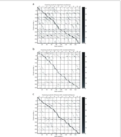
clusters using the scikit-learn software package [36]. We then analysed the way in which clusters correspond to states. The results of the analysis of the raw features are shown in Figure 8a. The horizontal axis in the figure corresponds to the 179 states, and the vertical axis to clus-ter numbers. The figure shows the association between
clusters and states. It can be seen that the exemplar clusters do associate to states, but there is a substantial amount of ‘confusions’. Figure 8b shows the result of the same clustering of the exemplars after applying an LDA transform to the exemplars, keeping all 135 dimensions. It can be seen that the LDA-transformed exemplars result in clusters that are substantially purer. Figure 8c shows the results of the same clustering on the 135-D features obtained from the LDA transform of sequences of 29 sub-sequent frames. Now, the cluster purity has increased further.
Although cluster purity does not guarantee high recog-nition performance, from Tables 1 and 2 it can be seen that the modulation spectrum features appear to capture substantial information that can be exploited by two very different classifiers.
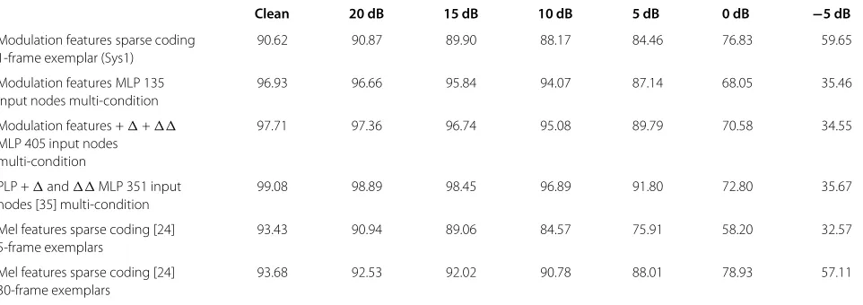
Table 2 Accuracies averaged over all noise types in test set A
Clean 20 dB 15 dB 10 dB 5 dB 0 dB −5 dB
Modulation features sparse coding 90.62 90.87 89.90 88.17 84.46 76.83 59.65
1-frame exemplar (Sys1)
Modulation features MLP 135 96.93 96.66 95.84 94.07 87.14 68.05 35.46
input nodes multi-condition
Modulation features ++ 97.71 97.36 96.74 95.08 89.79 70.58 34.55
MLP 405 input nodes multi-condition
PLP +andMLP 351 input 99.08 98.89 98.45 96.89 91.80 72.80 35.67
nodes [35] multi-condition
Mel features sparse coding [24] 93.43 90.94 89.06 84.57 75.91 58.20 32.57
5-frame exemplars
Mel features sparse coding [24] 93.68 92.53 92.02 90.78 88.01 78.93 57.11
30-frame exemplars
Accuracies (averaged over all noise types in test set A) obtained with Sys1 (SC system operating on 135-D modulation spectrum features), MLP classifiers (on same
features without and withs ands), MLP classifier on PLP features withs ands [35], SC classifier on Mel spectra [24] using 5- and 30-frame windows,
Z 1 2 3 4 5 6 7 8 9 O si l
State number s
Cluster number
s
Clustering results for single frame raw features
a
b
c
20 40 60 80 100 120 140 160
50
100
150
200
250
300
350
400
450
500
0 10 20 30 40 50 60
Z 1 2 3 4 5 6 7 8 9 O si l
Clustering results for single frame LDA−transformed features
State number s
Cluster number
s
20 40 60 80 100 120 140 160
50
100
150
200
250
300
350
400
450
500
0 10 20 30 40 50 60
Z 1 2 3 4 5 6 7 8 9 O si l
State number s
Cluster number
s
Clustering results for 29 frames LDA−transformed features
20 40 60 80 100 120 140 160
50
100
150
200
250
300
350
400
450
500
0 10 20 30 40 50 60
Figure 8Clustering results.(a)Single-frame raw features.(b)Single-frame LDA-transformed features.(c)The 29-frame LDA-transformed features.
3.2 Results obtained with the SC system
Table 1 summarizes the recognition accuracies obtained with six different systems, all of which used the SC approach to estimate state posterior probabilities. Four of these systems use the newly proposed modulation
spectrum features, while the remaining two describe the results using Mel-spectrum features as obtained in research done by Gemmeke [24].
frame of a modulation spectrum analysis by converting the exemplar weights obtained with the sparse classifica-tion system already yields quite promising results. Indeed, from a comparison with the results obtained with the orig-inal SC system using five-frame stacks in [24], it appears that the modulation spectrum features outperform stacks of five Mel-spectrum features in all but one condition. The conspicuous exception is the clean condition, where
the performance ofSys1is somewhat disappointing. Our
Sys1 performs worse than the system in [24] that used 30-frame exemplars. From the first and second rows, it can be inferred that transforming the features such that the discrimination between the 179 states is optimized is harmful for all conditions. Apparently, the transform learned on the basis of 17.148 exemplars does not gen-eralize sufficiently to the bulk of the feature frames. In section 4 we will propose an alternative perspective that puts part of the blame on the interaction between LDA and SC.
3.2.1 The representation of the temporal dynamics
In [20,24] the recognition performance in AURORA-2 was compared for exemplar lengths of 5, 10, 20, 30 frames. For clean speech, the optimal exemplar length was around ten frames and the performance dropped for longer
exemplars; at SNR= −5 dB, increasing exemplar length
kept improving the recognition performance and the opti-mal length found was the longest that was tried (i.e. 30). Longer windows correspond with capturing the effects of lower modulation frequencies. The trade-off between clean and very noisy signals suggests that emphasizing long-term continuity helps in reducing the effect of noises that are not characterized by continuity, but using 300-ms exemplars may not be optimal for covering shorter-term variation in the digits. From the two bottom rows in Table 1, it can be seen that going from 5-frame stacks to 30-frame stacks improved the performance for the nois-iest conditions very substantially. From the second and third rows in that table, it appears that the performance gain in our system that used 29-frame features (covering 72.5 ms) is nowhere near as large. However, due to the problems with the generalizability of the LDA transform
that we already encountered inSys2, it is not yet possible
to draw conclusions from this finding.
A potentially important side effect of using exemplars consisting of 30 subsequent frames in [20,24] was that the conversion of state activations to state posterior proba-bilities involved averaging over 30 frame positions. This diminishes the risk that a ‘true’ state is not activated at all. Our system approximates a feature frame as just one sum of exemplars. If an exemplar of a ‘wrong’ state hap-pens to match best with the feature frame, the Lasso procedure may fill the gap between that exemplar and the feature frame with completely unrelated exemplars. This
can cause gaps in the traces in the state probability lat-tice that represent the digits. This effect is illustrated in Figure 7a, which shows the state activations over time of the digit sequence ‘3 6 7’ at 5-dB SNR for the state proba-bilities in Sys1. The initial fricative consonants /θ/ and /s/ and the vowels /i/ and /I/ in the digits ‘3’ and ‘6’ are acous-tically very similar. For the second digit in the utterance, this results in somewhat grainy, discontinuous, and largely parallel traces in the probability lattice for the digits ‘3’ and ‘6’. Both traces more or less traverse the sequence of all 16 required states. The best path according to the Viterbi decoder corresponds to the sequence ‘3 3 7’, which is obviously incorrect.
3.2.2 Results based on fusing nine modulation bands
In Sys1, Sys2, and Sys3, we capitalize on the assump-tion that the sparse classificaassump-tion procedure can harness the differences between speech and noise in the modu-lation spectra without being given any specific informa-tion. In [32] it was shown that it is beneficial to ‘help’ a speech recognition system in handling additive noise by fusing the results of independent recognition oper-ations on non-overlapping parts of the spectrum. The success of the multi-band approach is founded in the finding that additive noise does not affect all parts of the spectrum equally severely. Recognition on sub-bands can profit from superior results in sub-bands that are only marginally affected by the noise. Using modula-tion spectrum features, we aim to exploit the different temporal characteristics of speech and noise, which are expected to have different effects in different modulation bands. Therefore, we conducted an experiment to inves-tigate whether combining the output of nine independent recognizers, each operating on a different modulation fre-quency band, will improve recognition accuracy. In each modulation frequency band, we have the output of all 15 gammatone filters; therefore, each modulation band ‘hears’ the full 4-kHz spectrum. The experiment was
con-ducted using the part of test set Athat is corrupted by
subway noise.
In our experiments we opted for fusion at the state posterior probability level: We constructed a single-state probability lattice for each utterance by means of a weighted sum of the state posteriors obtained from the individual SC systems. In all cases we fused the probability estimates of Sys1, which operates with 135-D exemplars with nine sets of state posteriors from SC classifiers that each operate on 15-D exemplars. Sys1 was always given a weight equal to 1. The weights for the nine modulation band classifiers were obtained using a genetic algorithm that optimized the weights on a small development set. The weights and WIP that yielded the best results in the
SNR conditions≤5 dB were applied to all SNR conditions.
Table 3 Weights obtained for combining the 15 gammatone filterbands in the multi-stream analysis
Fc(Hz) 0 2 3 4 5 6 8 10 16
GA −0.0172 −0.0921 0.0001 −0.0103 −0.223 −0.0336 −0.0072 −0.0625 0.201
GA, weights obtained with a genetic algorithm.
From row 4 (Sys4) in Table 1, it can be seen that
fus-ing the state likelihood estimates from the nine individual modulation filters with the state likelihoods from the full modulation spectrum deteriorates the recognition accu-racy for all but two SNRs. From Table 3 it appears that the Genetic Algorithm returns very small weights for all nine modulation bands. This strongly suggests that the individual modulation bands are not able to highlight spe-cific information that is less easily seen in the complete modulation spectrum.
A potentially very important concomitant advantage of fusing the probability estimates from the 135-D system and the nine 15-D systems is that the fusion process may make the probability vectors less sparse, thereby reduc-ing the risk that wrong states are bereduc-ing promoted. This is illustrated in Figure 7b, where it can be seen that the state probability traces obtained from the fusion of the full 135-D system and the weighted sub-band systems suffer less from competing ‘ghost traces’ of acoustically simi-lar competitors that traverse all 16 states of the wrong digit: Due to the lack of consensus between the multi-ple classifiers, the trace for the wrong digit ‘3’, which is clearly visible in Figure 7a, has become less clear and more ‘cloud-like’ in Figure 7b. As a consequence, the digit string is now recognized correctly as ‘3 6 7’. However, from the results in Table 1, it is clear that on average the impact of making the probability vectors less sparse by means of fusing modulation frequency sub-bands is negligible.
3.3 Results obtained with MLPs
We trained four MLP systems for computing state poste-rior probabilities on the basis of the modulation spectrum features, two using only clean speech and two using the multi-condition training data. We increased the number of hidden nodes, starting with 200 hidden nodes up to 1,500 nodes. In all cases the eventual recognition accuracy kept increasing, although the rate of increase dropped substantially. Additional experiments showed that further increasing the number of hidden nodes no longer yields improved recognition results. For each number of hid-den nodes, we also searched for the WIP that would
provide optimal results for the cross-validation set (cf.
section 2.7). We found that the optimal accuracy in the different SNR conditions was obtained for quite different values of the WIP. Training on multi-condition data had a slight negative effect on the recognition accuracy in the clean condition, compared to training on clean data only.
However, as could be expected, the MLPs trained on clean data did not generalize to noisy data.
Table 2 shows the results obtained with SC systems operating on modulation spectrum and Mel-spectrum features and the MLP-based systems trained with
multi-condition data. It can be seen that adding and
features to the ‘static’ modulation spectrum features increases performance somewhat, but by no means to the
extent that addingand features improves
perfor-mance with Mel-spectrum or PLP features [12,13]. The two systems that used modulation spectrum fea-tures perform much worse on clean speech than the
MLP-based system that used nine adjacent 10-ms PLP++
features [37]. This suggests that the modulation spectrum features fail to capture part of the dynamic information that is represented by the speed and acceleration features derived from PLPs. Interestingly, that information is not restored by adding the regression coefficients obtained with stacks of modulation frequency features. In the nois-ier conditions, the networks trained with modulation fre-quency features derived from the multi-condition training data approximate the performance of the stacks of nine extended PLP features.
4 Discussion
In this paper we introduced a basic implementation of a noise-robust ASR system that uses the modulation spec-trum, instead of the short-time spectrum to represent noisy speech signals, and sparse classification to derive state probability estimates from time samples of the mod-ulation spectrum. Our approach differs from previous attempts to deploy sparse classification for noise-robust ASR. The first difference is the use of the modulation spectrum and the second is that the exemplars in our system are constituted by individual frames, rather than by (long) sequences of adjacent frames in [20,24], which needed such sequences to effectively cover essential infor-mation about continuity over time that comes for free in the modulation spectrum, where individual frames cap-ture information about the dynamic changes in the short-time spectrum. Our unadorned implementation yielded recognition accuracies that are slightly below the best results in [20,24], but especially the fact that our system
yielded higher accuracies in the −5-dB SNR condition
and posterior state probability estimation, we will discuss the features and the estimators separately - to the extent possible.
4.1 The features
In designing the modulation spectrum analysis system, a number of decisions had to be made about implemen-tation details. Although we are confident that all our decisions were reasonable (and supported by data from the literature), we cannot claim that they were optimal. Most data in the literature on modulation spectra are based on perception experiments with human subjects, but more often than not these experiments use auditory stimuli that are very different from speech. While the results of those experiments surely provide guidance for ASR, it may well be that the automatic processing aimed at extracting the discriminative information is so differ-ent from what humans do that some of our decisions are sub-optimal. Our gammatone filterbank contains 15 one-third octave filters, which have a higher resolution in
the frequencies<500 Hz than the Mel filterbank that is
used in most ASR systems. However, initial experiments in which we compared our one-third octave filterbank with a filterbank consisting of 23 Mel-spaced gammatone filters, spanning the frequency range of 64 to 3,340 Hz did not show a significant advantage of the latter over the former. From the speech technology’s point of view, this may seem surprising because the narrow-band filters of the one-third octave filterbank in the low frequen-cies may cause interactions with fundamental frequency, while the relatively broad filters in the higher frequencies cannot resolve formants. But from an auditory system’s point of view, there is no such surprise, since one-third octave filters are compatible with most, if not all, out-comes of psycho-acoustic experiments. This is also true for experiments that focused on speech intelligibility [1].
For the modulation filterbank, it also holds that the design is partly based on the results of perception experi-ments [19]. Our modulation frequency analyser contained filters with centre frequencies ranging from 0 to 16 Hz. From [30] it appears that the modulation frequency range of interest for ASR is limited to the 2- to 16-Hz region. Therefore, here too we must ask whether our design is optimal for ASR. It might be that the spacing of the modulation filters in the frequency band that is most important for human speech intelligibility is not optimal for automatic processing. However, as with the gamma-tone filters, it is not evident why a different spacing should be preferred. It might be necessary to treat modulation
frequencies≤1 Hz, which are more likely to correspond to
the characteristics of the transmission channel, different than modulation frequencies that might be related to articulation. One might think that the very low modula-tion frequencies would best be discarded completely in
the AURORA-2 task, where transmission channel char-acteristics do not play a role. However, experiments in which we did just that yielded substantially worse results. Arguably, the lowest modulation frequencies help in dis-tinguishing time intervals that contain speech from time intervals that contain only silence or background noise. We decided to not include modulation filters with centre
frequencies >16 Hz. This implies that we ignore almost
all information related to the periodicity that character-izes many speech sounds. However, it is well known that the presence of periodicity is a powerful indicator of the presence of speech in noisy signals and also, in case the background noise consists of speech from one or more interfering speakers, a powerful means to separate the tar-get speech from the background speech. In future experi-ments we will investigate the possibility of adding explicit information about the harmonicity of the signals to the feature set.
The experiments with the MLP classifiers for obtaining state posterior probabilities from the modulation spec-trum features confirm that the modulation specspec-trum fea-tures capture most of the information that is relevant for speech decoding. Still, the WERs obtained with the MLPs were always inferior to the results obtained with stacks of
nine conventional PLP features that include and
features, especially in the cleanest SNR conditions. Although the modulation spectrum features are perform-ing quite well in noisy conditions, in cleaner conditions their performance is worse than the classical PLP features.
Addings ands, computed as linear regressions over
90 ms windows, to the modulation spectrum features does not improve performance nearly as much as adding speed and acceleration to MFCC or PLP features. This suggests that our modulation spectrum features are suboptimal with respect to describing the medium-term dynamics of the speech signal. The time windows associated with the modulation frequency filters with the lowest cen-tre frequencies is larger than 500 ms. As a consequence, time derivatives computed over a window of 90 ms for these slowly varying filter outputs is not likely to carry much additional information. We suspect that the fea-tures in the lowest modulation bands play too heavy a role. If we want to optimally exploit the redundancy in the different modulation frequency channels when part of them gets obscured by noise, information about relevant speech events (such as word or syllable onsets and off-sets) should ideally be represented equally well by their temporal dynamics in all channels.
the modulation filters (rather than the gammatone fil-ters) already showed a substantial beneficial effect. The additional high-pass filtering that is performed in the compression/adaptation network (which should only be applied to the output of the gammatone filters) is expected to have a further beneficial effect in that it implements the medium-term dynamics that we seem to be missing at the moment. Including the adaptation stage is also expected to enhance the different dynamic characteristics of speech and many noise types in the modulation frequency bands. If this expectation holds, the absence of a proper adapta-tion network might explain the failure of the nine band fusion system.
4.2 The classifiers
Visual inspection of traces of state activations as a func-tion of time obtained with the SC system suggested that the similarity between adjacent feature vectors was much higher than the similarity between adjacent state activa-tion vectors. Figure 9 shows scatter plots of the relaactiva-tion between the similarity between adjacent feature vectors and the corresponding state probability vectors. It can be seen that the Pearson correlation coefficient between adjacent feature frames is very high, which is what one
would expect, given the high sampling rate. It is also evi-dent, and expected, that the variance increases as the SNR decreases. However, the behaviour of the state probabil-ity vectors is quite different. While for part of the adjacent vectors it holds that they are very similar (the pairs with a similarity close to one, represented by the points in the upper right-hand corner of the panels), it can be seen that there is a substantial proportion of adjacent state probabil-ity vectors that are almost orthogonal. We believe that this discrepancy is related to the difference between sparse coding (reconstruction of an observed modulation spec-trum in terms of a linear combination of exemplars), what it is that the Lasso solver does, and sparse classification (estimating the probability of the HMM state underly-ing the observed modulation spectrum), which is our final goal. The frames that represent an unknown (noisy) speech signals are all decoded individually; for each frame the Lasso procedure starts from scratch. If occasionally a speech atom related to a wrong state or an atom from the noise dictionary happens to match best with an input frame, this can have a very large impact on the resulting state activation vector. Lasso can turn a close similarity between an input frame and exemplars related to the true state at the feature level into a close-to-zero probability
0 0. 5 1 −0. 5
0 0. 5 1
1 frame
0 0. 5 1 −0. 5 0 0. 5 1 SNR=20 2 frame
0 0. 5 1 −0. 5
0 0. 5 1
3 frame
0 0. 5 1 −0. 5
0 0. 5 1
4 frame
0 0. 5 1 −0. 5
0 0. 5 1
5 frame
0 0. 5 1 −0. 5
0 0. 5 1
0 0. 5 1 −0. 5
0 0. 5 1 SNR=15
0 0. 5 1 −0. 5
0 0. 5 1
0 0. 5 1 −0. 5
0 0. 5 1
0 0. 5 1 −0. 5
0 0. 5 1
0 0. 5 1 −0. 5
0 0. 5 1
Correlation of state activations in frames with distance
N
0 0. 5 1 −0. 5
0 0. 5 1 SNR=10
0 0. 5 1 −0. 5
0 0. 5 1
0 0. 5 1 −0. 5
0 0. 5 1
0 0. 5 1 −0. 5
0 0. 5 1
0 0. 5 1 −0. 5
0 0. 5 1
0 0. 5 1 −0. 5
0 0. 5 1 SNR=5
0 0. 5 1 −0. 5
0 0. 5 1
0 0. 5 1 −0. 5
0 0. 5 1
0 0. 5 1 −0. 5
0 0. 5 1
0 0. 5 1 −0. 5
0 0. 5 1
0 0. 5 1 −0. 5
0 0. 5 1 SNR=0
0 0. 5 1 −0. 5
0 0. 5 1
0 0. 5 1 −0. 5
0 0. 5 1
0 0. 5 1 −0. 5
0 0. 5 1
0 0. 5 1 −0. 5
0 0. 5 1
0 0. 5 1 −0. 5
0 0. 5 1 SNR= −5
0 0. 5 1 −0. 5
0 0. 5 1
correlation of features in frames with distance N
0 0. 5 1 −0. 5
0 0. 5 1
0 0. 5 1 −0. 5
0 0. 5 1
of the ‘correct’ state in the probability vector because an exemplar related to another state (or noise) happened to match slightly better.
The substantial deterioration of the recognition perfor-mance with LDA-transformed features came as a surprise, not in the last place because we have seen that cluster purity increases after LDA transform. The fact that we see a negative effect of the transform already for clean speech suggests that the transformation matrix learned from the exemplar dictionary does not generalize well to the con-tinuous speech data. While the correlation between the raw features in adjacent frames was very close to one in the raw features, the average Pearson correlation coefficient between adjacent frames dropped to about 0.75 after the LDA transform. The LDA transformation maximizes the differences among the 179 states, regardless of whether states are actually very similar or not. Distinguishing adja-cent states in the digit word ‘oh’ is equally important as distinguishing the eighth state of oh from the first state of ‘seven’. Exaggerating the differences between adjacent frames, because these may relate to different states, is likely to aggravate the risk that Lasso returns high activa-tions for a wrong state because an exemplar assigned to that state happens to fit the frame under analysis best. In addition, the LDA transform affects the relations between the distributions of the features. Because we believe that the feature normalization applied to the raw modula-tion spectrum features yielded the best performance since it conforms with the mathematics in Lasso, we applied the same normalization to the LDA-transformed features. We did not (yet) check whether a different normaliza-tion could improve the results. The comparison between the single-frame LDA-transformed and 29-frame features that are reduced to 135-D features by means of an LDA-transform shows that adding a more explicit representa-tion of the time context only improves the recognirepresenta-tion accuracy in the 10- and 5-dB SNR conditions; in all other conditions, the results obtained with single-frame fea-tures are better. We believe that this finding is related to the difficulty of representing medium-term speech dynamics in the present form of the modulation spectrum features.
We experimented with LDA in order to be able to explicitly include additional information about temporal dynamics. In the present implementation, with its 400-Hz frame rate, a stack of 29 adjacent frames covers a time interval of 72.5 ms, resulting in 3,915-D feature vectors. However, the 400-Hz frame rate does not seem to be nec-essary. Preliminary experiments with low-pass filtering the Hilbert envelopes of the outputs of the gammatone fil-ters with a cut-off frequency of 50 Hz and a frame rate of 100 Hz yielded equal WER results. This opens the possi-bility of covering time spans of about 70 ms by concate-nating only nine frames. However, an experiment in which
we decoded the clean speech with exemplars consisting of nine subsequent 10-ms frames did not yield accuracies better than what we had obtained with single-frame fea-tures. This corroborates our belief that the medium-term dynamics is not sufficiently captured by our modulation spectrum features.
The success of the MLP classifiers that is apparent from Table 2 shows that sparse classification is not the only way for estimating state posterior probabilities from modula-tion spectrum features. In fact, the MLP classifier yielded consistently better results than the SC classifier in the SNR conditions covered by the training data. However, in the
0- and−5-dB SNR conditions, which are not present in
the multi-condition training, the SC classifier yielded bet-ter performance. This raises the question whether it is possible to add supervised learning to the design of an SC-based system without sacrificing its superior general-ization to unseen conditions.
In [20] and [24] it is mentioned that they failed to improve the performance of their sparse coding systems by machine learning techniques in the construction of the exemplar dictionaries. However, the cause of the failure was not explained. It may well be that the situation with single-frame modulation spectrum exemplars is different from 30-frame Mel-spectrum exemplars so that clever dictionary learning might be beneficial. We have started experiments with fast dictionary learning along the lines set out in [39]. Our first results suggest that there are two quite different issues that must be tackled. The first issue relates to the cost function used in creating the optimal exemplars. Conventional approaches to dictionary learn-ing use the difference between unknown frames and their approximation as a weighted sum of exemplars as the cri-terion to minimize. While this cricri-terion is obviously valid
in sparse coding applications, it is not the criterion of
choice in sparseclassification. In the latter application, the exemplars carry information about the states (the classes) that they represent, and this information should enter into the cost function, for example, in the form of the require-ment that individual exemplars are promoted for frames that do correspond to a certain state (or set of acoustically similar states).
The second issue is that the mapping from state
activa-tions returned by somesolverto state posterior
probabil-ities is less straightforward than was implemented in [20] and [24] and in this paper. There is a need for includ-ing some learninclud-ing mechanisms that can find the optimal mapping from a complete set of state activations to a set of state posteriors. It is quite possible that there will be interactions between enhanced dictionary learning and learning the mapping from activations to probabilities. The challenge here is to find strategies that do not fall into the trap that we have seen in our experiments with
the conditions for which training material was available but at the cost of a diminished generalization to unseen conditions.
An issue that surely needs further investigation in the construction of the dictionary is the selection of the noise exemplars. So far, noise exemplars were extracted quasi-randomly from the four noise types that were used in
creating the multi-condition training set in AURORA-2.
It is quite likely that the collection of noise exemplars is much more compactly distributed in the feature space than the speech exemplars because the variation in the noise signals is less than in the speech signals. The gen-eralization to other noise types can be improved by sam-pling the exemplars from a wider range of noises, for example all noise types that are available in the NOISEX CD-ROM [40]. However, we think that the most impor-tant issue in the construction of the noise exemplar dic-tionary is the need for avoiding overlap between noise and speech exemplars. In the Lasso procedure, it is difficult - if not impossible - to enforce a preference for speech atoms over noise atoms. If a noise exemplar that is very sim-ilar to a speech exemplar happens to fit best, this may give rise to suppressing relevant speech information. It might be beneficial to not simply discard all noise exem-plars activations but rather to include these, along with the activations of the speech exemplars, in a procedure that learns the mapping from activations to state posteri-ors that optimizes recognition performance. An approach in which all activations are used in estimating the even-tual posterior probabilities would be especially important in cases where noise and speech are difficult to distinguish in terms of spectro-temporal properties, such as in bab-ble noise or if the ‘noise’ consists of competing speakers. These cases will surely require additional processing, for example, aimed at tracking continuity in pitch, in addition to continuity in the modulation spectrum.
5 Conclusions
In this paper we presented a novel noise-robust ASR sys-tem that uses the modulation spectrum in combination with a sparse coding approach for estimating state prob-abilities. Importantly, in its present implementation, the system does not involve any form of learning/training. The best recognition accuracies obtained with the novel system are slightly below the results that have been obtained with conventional engineering systems. We have also sketched several research lines that hold the promise of improving the results and, at the same time, to advance our knowledge of those aspects of the human auditory system that are most important for ASR. We have shown that the output of a modulation spectrum analyser that does not involve any form of conversion to the equivalent of a short-time power spectrogram is able to exploit the spectro-temporal continuity constraints that are typical
for speech and which are a prerequisite for noise robust ASR. However, we also found that the representation of medium-term dynamics in the output of the modulation spectrum analyser must be improved. With respect to the sparse coding approach to estimate state posterior prob-abilities, we have found that there is a fundamental dis-tinction between sparse coding, where the task is to find the optimal representation of an unknown observation in a very large dimensional space, and sparse classification, where the task is to obtain the best possible estimates of the posterior probability that an unknown observation belongs to a specific class. In this context one challenge for future research is developing a procedure for dictionary learning that uses state posterior probabilities, in addition to or rather than reconstruction error, as the cost function. The second challenge is finding a procedure for learn-ing a mapplearn-ing from state activations to state posterior probabilities that provides the same excellent generaliza-tion to unseen condigeneraliza-tions that has been found with sparse coding.
Endnote
aThe software used for implementing the modulation
frequency analyser was adapted from Matlab code that was kindly provided by Søren Jørgensen [41]. Some choices that are somewhat unusual in speech technology, such as the 400-Hz frame rate, were kept.
Competing interests
The authors declare that they have no competing interests.
Acknowledgements
Part of this research has been funded with support from the European Commission under contract FP7-PEOPLE-2011-290000 to the Marie Curie ITN INSPIRE. We would like to thank Hugo Van hamme and Jort Gemmeke for discussing feature extraction and sparse coding issues and Søren Jørgensen for making available the Matlab code for implementing the modulation spectrum analyser. Finally, we owe thanks to two anonymous reviewers, whose comments greatly helped to improve the paper.
Author details
1Amirkabir University of Technology, Hafez 424, 15875-4413 Tehran, Iran. 2Centre for Language Studies, Radboud University Nijmegen, Erasmusplein 1, 6525HT Nijmegen, Netherlands.
Received: 9 January 2014 Accepted: 20 August 2014
References
1. R Drullman, JM Festen, R Plomp, Effect of temporal envelope smearing on speech reception. J. Acoust. Soc. Am.95, 1053–1064 (1994)
2. H Hermansky, inProceedings of IEEE Workshop on Automatic Speech Recognition and Understanding. The modulation spectrum in the automatic recognition of speech (Santa Barbara, 14–17 December 1997), pp. 140–147
3. X Xiao, ES Chng, H Li, Normalization of the speech modulation spectra for robust speech recognition. IEEE Trans. Audio Speech Lang. Process.16(8), 1662–1674 (2008)