Enhanced Random Forest Algorithms for Partially Monotone Ordinal Classification

The Thirty-Third AAAI Conference on Artificial Intelligence (AAAI-19)

Enhanced Random Forest Algorithms

for Partially Monotone Ordinal Classification

Christopher Bartley, Wei Liu, Mark Reynolds

Computer Science and Software Engineering University of Western Australia, Perth, Australia

[email protected],{wei.liu,mark.reynolds}@uwa.edu.au

Abstract

One of the factors hindering the use of classification models in decision making is that their predictions may contradict expectations. In domains such as finance and medicine, the ability to include knowledge of monotone (nondecreasing) relationships is sought after to increase accuracy and user sat-isfaction. As one of the most successful classifiers, attempts have been made to do so for Random Forest. Ideally a so-lution would (a) maximise accuracy; (b) have low complex-ity and scale well; (c) guarantee global monotoniccomplex-ity; and (d) cater for multi-class. This paper first reviews the state-of-the-art from both the literature and statistical libraries, and identi-fies opportunities for improvement. A new rule-based method is then proposed, with a maximal accuracy variant and a fasterapproximate variant. Simulated and real datasets are then used to perform the most comprehensive ordinal classi-fication benchmarking in the monotone forest literature. The proposed approaches are shown to reduce the bias induced by monotonisation and thereby improve accuracy.

Introduction

This paper concernsmonotone prior knowledge. A mono-tone (or non-decreasing) relationship between X and Y means that an increase in X should not lead to a decrease in Y. For example, a house with three bedrooms should not be cheaper than one with two bedrooms (all other factors constant). Monotonicity between input variable (feature)xj

and output variableymay thus be defined:

For an increase inxj, response variableyshould not

decrease (all other variables held constant).

Monotonicity can be defined when the model output is or-dered, including ordinal classification, which seeks to as-sign objects to two or more ordered classes (but where the distancesbetween classes are irrelevant). Examples include credit ratings (AA, A, BB, ...), or cancer diagnosis (No/Yes). This paper focuses on Random Forest (RF) style tree en-sembles with independent large (unpruned) trees (Breiman 2001). RF is one of the most popular classifiers, achieving both high accuracy and ease of use. It’s competitive accu-racy was somewhat surprisingly reasserted in the compre-hensive 2015 comparison by Fernandez et al. of 179 classi-fiers against 121 datasets (Fernandez-Delgado et al. 2014),

Copyright © 2019, Association for the Advancement of Artificial Intelligence (www.aaai.org). All rights reserved.

where it was the highest ranked model family. We note that this comparison omitted deep learning approaches, to which monotonicity has recently been extended (You et al. 2017). However, there remains a significant use case for RF for smaller datasets, users with less expertise, where computa-tional power is limited and where solution time is critical.

However, despite its popularity, for sensitive domains like finance and medicine where users want to know how the model works, RF’s lack ofcomprehensibilityis a problem. As a result the ability to definemonotone featuresis popu-larly requested and implemented in many libraries such as

R’sGBMandArboristandXGBoost. This helps achieve quality control(ensuring a model behaves ‘sensibly’), satis-faction ofuser requirements(e.g. known medical risk fac-tors) and improved comprehensibility. Although still not fully comprehensible, features may now be categorised as increasing or decreasing, with magnitude estimated by vari-able importance measures. This latter is particularly com-pelling given the recently enacted GDPR legislation1_{, which}

confers ondata subjectsthe right to ‘meaningful information about the logic involved’ in ‘automated decision making’.

This paper therefore pursues the twin goals of compre-hensibility and accuracy. We first review the state-of-the-art in monotone random forest, with extensions where neces-sary to multi-class. This review for the first time combines both previous literatureandapproaches in popular statistical libraries that are absent from the literature.

A key limitation of some approaches is that monotonicity is increasedlocally, but not guaranteedglobally. There is a big difference between being able to claim that an algorithm usuallycomplies, and that it categoricallyalwayscomplies. The latter is surely preferable. Of the techniques that do achieve global monotonicity, we show their mechanisms can result in sub-optimal monotonisation (high loss/bias). Since RF primarily improves accuracy byvariancereduction, this introducedbiascannot be corrected and accuracy suffers.

We thus propose a method with global monotonicity and minimal monotonisation loss. Examples and simulation demonstrate lower monotonisation loss, and experiments on 17 real datasets show a compelling increase in accuracy. The algorithm is available atgithub2.

1

https://eur-lex.europa.eu/eli/reg/2016/679/oj

2

Monotone Ordinal Classification and Random

Forest

The classification task is to build a function f : X → Y to predict the classy ∈ Y given input pointx ∈ X, where Y={c1, c2, ..., cC}. The classifierfis built using a training

set ofN samples{(xi, yi)}, i= 1..N,xi ∈ X, yi ∈ Y. The

ordinal classification task adds a total order on the classes to be predictedc1 ≺c2 ≺... ≺cC. Unlike regression, the

distance between classes is undefined.

Partially monotone ordinal classifiers allow the user to specify that one or more of the features in X has a non-decreasing(non-increasing) impact on the output class. For clarity we split the input space _Rp _{into X × Z, X ⊆}

Rpx_{,Z ⊆}

Rpz_{, whereX contains thep}

xmonotone features,

andZthepznon-monotone features (p=px+pz). Thus:

Definition 1 Partial Dominance

Given(x,z),(x0,z0)∈Rpx_×

Rpz_{, the partial order} X is:

(x,z)X (x0,z0)⇔xx0∧z=z0 (1)

As a partial order,X is transitive, anti-symmetric and

re-flexive. We can now define a partially monotone function: Definition 2 Partially Monotone Function

FunctionF :X × Z → Y,X ⊆Rpx_{,Z ⊆}

Rpz _ismonotone increasingin the features ofX (i.e.{1..px}) if:

xx0⇒F(x,z)≤F(x0,z),∀x,x0∈ X,z∈ Z (2)

Random Forest (RF)The RF algorithm was proposed by Breiman in 2001 and emerges from the tree ensemble tech-niques developed in the late 1990s (Breiman 2001). Each component tree differs from the well-known CART algo-rithm due to: first, each tree is trained on abootstrap sam-pleof the training data (‘bagging’); second, as each tree is inducted only arandom subsetof mtry of the features are

considered for the best split. The greatly improved accu-racy achieved by RF is due to the variance reducing impact of bagging on unbiased predictors (unpruned trees) that are decorrelated (due tomtry) (Hastie, Tibshirani, and J. 2009).

As will become apparent, it is therefore crucial to minimise bias when monotonising the trees, because bagging (unlike boosting) cannot correct for it.

Existing Monotone RF Approaches

This section describes state-of-the-art monotone tree ensem-bles and critiques them as they apply to RF. To our knowl-edge this is the most comprehensive account in the literature, and includes approaches from statistical libraries that are not mentioned in the literature (split-wise constraints and the

XGBoostapproach) or exist independently within different branches (Isotonic Classification Trees vs Rule Reshaping). First Order Stochastic Dominance RF (FSD-RF)The na¨ıve solution to monotonising a tree is to constrain each branch to prohibit nonmonotone splits. For regression trees this corresponds to ensuring the means of proposed leaf nodes correspond to the leaf partial order (for splits on

monotone features). This technique is implemented for ex-ample in the GBM3 and Arborist4 libraries for R. For binary classification the constraint is simply applied to

Pr(y=+1)rather than the leaf mean.

We extend this to multi-class using First-order Stochas-tic Dominance (FSD). FSD is a partial order over probabil-ity distributions, and is expressed in terms of the cumulative probability distribution (cdf). For ordinal classesc∈ {1..C} the cdfFA(c∗) =P r(c≤c∗)has first order stochastic dom-inance over FB(c∗)ifFA(c∗) ≤ FB(c∗) ∀c∗ ∈ {1..C}.

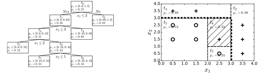
FSD-RF thus simply prohibits non-FSD branch splits. The advantage of split-wise constraints is that it has vir-tually no computational overhead. The disadvantage is that monotonicity is not necessarily global. For example Figure 1 shows a tree that is notglobally monotone despite each branch satisfying constraints on x1 and x2: when nodet6 splits onx2≤3, the createdt7predictsy =-1and is non-monotone in bothx1andx2.

Monotone Induction Decision Trees (MID-RF) Gonz´alez, Herrera, and Garcia (2015) propose a forest based on Ben-David’s MID Trees (Ben-David 1995). MID modifies tree induction by choosing the split to minimise not just entropyE, butT =E+RA, whereAis the ‘order ambiguity’, and R ≥ 0 is a weighting factor.Apenalises splits that result in nonmonotone branch pairs. MID-RF randomisesR ∈ {1,2, ..., Rlim}, Rlim= 100for each tree

and also prunes the ensemble to retain only thex = 50%

most monotone trees. MID-RF has the advantage of natively allowing multi-class classification.

MID-RF does not achieve global monotonicity since the leaf-wise non-monotonicity penalty discourages but does not prohibit nonmonotone splits. The second limitation is complexity. Each branch split compares all possible splits against all other existing leaves to calculateA, resulting in O(ntreemtrypN˜3)complexity, wherentree is the number

of trees,mtryis the number of random features considered,

pis the number of features, andN˜ is the number of unique points in a bootstrap sample (≈0.632N).

Partially Monotone Random Forest (PM-RF)Bartley, Liu, and Reynolds (2016) monotonise RF by introducing training point weightss={si|i= 1..N}and using convex

optimisation to calculate them such that the ensemble com-plies withKdiscrete constraints(_∼xk,˜xk)designed to correct

nonmonotonicities while minimisingPN_i=1(si− _N1)2. The

disadvantages are similar to MID-RF: although constraint compliance is assured global monotonicity is not, and solv-ing the quadratic program is approximatelyO(N3_).

PM-RF is a binary classifier, and to extend it to multi-class we use the monotone ensembling by Kotlowski (Kot-lowski 2008). Lethc(x) = 1[y < c]be a binary classifier that distinguishesclass less thanc fromclass greater than or equal toc, where1[condition] = 1ifconditionelse0. Then multi-class classifierh:X → Y(Y ={1,2, ..., C}) is given by:

3

https://cran.r-project.org/web/packages/gbm/index.html

4

t2 p+= 0.0

t3 p+= 1.0 t1 p+= 0.2

x1 3

t5 p+= 0.57

t7 p+= 0.0

t8 p+= 1.0 t6 p+= 0.67

x2 3 t4 p+= 0.6

x1 4 t0

p+= 0.47 x2 2

Yes No

0.0 1.0 2.0 3.0 4.0 5.0

x

1

0.0 1.0 2.0 3.0 4.0 5.0

x

2 t2 p+= 0.0

t3 p+= 1.0

t5 p+= 0.57

t7 p+= 0.0

t8 p+= 1.0

Figure 1: Split Constrained Tree Example (monotone inx1,x2). Left: Tree. Right: Leaf partitions shown dotted, class boundary bold dotted. Positive class+, negative◦.p+denotesPr(y=+1). Note nonmonotonet7, despite splits respecting monotonicity.

t5

p+∈[0.0,0.24] p+= 0.12

t7

p+∈[0.24,0.33] p+= 0.24

t8

p+∈[0.33,0.43] p+= 0.43

t6

p+∈[0.24,0.43] p+= 0.43

x2 1

t3

p+∈[0.0,0.43] p+= 0.21

x1 2

t4

p+∈[0.43,0.68] p+= 0.68

t1

p+∈[0.0,0.68] p+= 0.38

x2 3

t2

p+∈[0.68,1.0] p+= 0.88

t0

p+∈[0.0,1.0] p+= 0.55

x1 3

Yes No

0.0 0.5 1.0 1.5 2.0 2.5 3.0 3.5 4.0

x

1

0.0

0.5

1.0

1.5

2.0

2.5

3.0

3.5

4.0

x

2

t

2

p+= 0.88

t

4

p+= 0.68

t

5

p+= 0.12

t

7

p+= 0.24

t

8

p+= 0.43

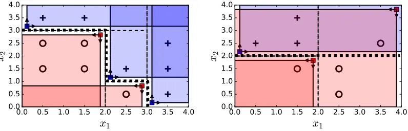
Figure 2: XGBoost Monotone Tree Example. Left: Tree. Right: Leaf partitions dotted, class boundary bold dotted. Positive class+, negative◦.p+denotesPr(y=+1). Notet8non-optimally predictsy=−1(p+ ≤0.5) due to inherited constraints.

h(x) = 1 +

C X

c=2

hc(x) (3)

Ifhc(x)are monotone,h(x)are monotone with L1 loss

bounded by the sum of the L1 loss ofhc(Kotlowski 2008).

XG-Boost Constrained Trees (XGM-RF) The popular

XGBoost(Chen and Guestrin 2016) uses a novel approach that combines split constraints withinherited leaf coefficient limits. At each split, the mean of the left and right coef-ficients is passed down as anupperlimit on future coeffi-cients to the left leaf, and alowerlimit to the right leaf (for binomial deviance these are the mean oflogit(Pr(y=+1))

rather than Pr(y=+1)). These inherited constraints are re-spected when greedily finding optimal leaf splits and effec-tively guarantee global monotonicity. This elegant approach has virtually no computational overhead while achieving globally guaranteed monotonicity.

The disadvantage is that this can severely reduce the in-sample accuracy of large trees (i.e. itbiases the tree away from the training data). Figure 2 shows how this occurs. The root nodet0passes an upper limit tot1ofp+≤0.68, which is reduced top+≤0.43when split to createt3. Then fromt3 onwards it is impossible to predicty=+1(p+ >0.5). Thus whent8(hatched) is created to extract the positive point, the

lowest loss solution allowed isp+=0.43, predictingy=-1. This is despite the factt8could predictp+=0.68without vi-olating monotonicity. In fact after depth≈2one branch will be constrained to predicty=+1, and one to predicty=-1.

In its original context (gradient boosting) this approach remains ideal because the trees are shallow (depth≈3),and any bias introduced by one tree can be corrected by subse-quent trees. In contrast, RF uses trees created from indepen-dent bootstrap samples (with no opportunity to correct intro-duced bias), and grows deep trees to near leaf purity (often having>40leaves and depth>6). This approach thus in-troduces bias that appears likely to reduce RF accuracy.

To extend this method to multi-class we cannot use stan-dard one-vs-rest (OVR) ensembling because the partial or-der is unclear (e.g. Class 2 vs Classes 1,3,4). Instead we use the Kotlowski ensembling (Kotlowski 2008), as outlined for PM-RF in (3).

t2

p+= 0.0

t3

p+= 1.0

t1

p+= 0.75

x2 2

t4

p+= 0.0

t0

p+= 0.43

x1 2

Yes No

0.0 0.5 1.0 1.5 2.0 2.5 3.0 3.5 4.0

x

1

0.0 0.5 1.0 1.5 2.0 2.5 3.0 3.5 4.0

x

2

_t2

p+, orig= 0.0 p+, iso= 0.0

t3

p+, orig= 1.0 p+, iso= 0.5

t4

p+, orig= 0.0 p+, iso= 0.5

Figure 3: Isotonic Classification Tree Example. Left: Tree. Right: Leaf partitions dotted, class boundary bold dotted. Positive class+, negative◦.p+denotesPr(y=+1). Best possible solution to isotonic relabelling isp+= 0.43for all leaves (i.e.yˆ=-1).

this leaf partial order. We note this is in effect theIsotonic Classification Trees (ICT) approach proposed by van de Kamp, Feelders, and Barile (2009), where it is also noted that the tree may be sequentially simplified to eliminate branches where both leaves predict the same class. Thus for ICT a relabelling/simplification cycle is repeated until all leaves are monotone with respect to each other. ICT also allows multi-class by using monotone ensembling based on FSD and selecting the lowest median to allow multi-class. Thus instead of the ‘rule reshaping’ approach we use ICT for each tree.

However, we observe this is likely to yield biased and sub-optimal monotonisation. Because the regression is limited to relabelling existing leaves, the monotonisation candidates are not always very good. This is illustrated in Figure 3. The original tree finds leaf purity with three leaves, with prob-abilitiesp+,orig. The regression must then respect the leaf

partial ordert2t3t4and the optimal and only solution isp+,iso = 0.43, universally predicting the majority class

(-1) and misclassifying thethree+points). The obvious so-lution (two nodesx2 ≤ 2andx2 >2), which would only misclassifyonepoint, is not possible by leaf relabelling be-cause the regression was given an unfortunate leaf partition. Another disadvantage of ICT (and rule reshaping) is that the solution to isotonic regression is typicallyO(N3_)for inte-rior point solutions to the quadratic program.

A New Method: Monotone Rule RF (MR-RF)

We now propose an approach to address the weaknesses above. MID-RF, PM-RF, and FSD-RF are unable to guaran-tee monotonicity. XGM-RF and ICT-RF do guaranguaran-tee global monotonicity, but both use mechanisms that are likely to lead to sub-optimal monotonisation.

We propose instead to convert the Random Forest to a rule ensemble in such a way as to ensure global monotonicity while reducing the introduced bias. First observe that binary RF can be considered as an additive rule ensemble (Bart-ley, Liu, and Reynolds 2016; Bonakdarpour et al. 2018). Splitting the input space into the monotone (x) and non-monotone (z), the classifier produced by tree ensembles can

be written as a weighted sum over all leaves of all trees:

F(x,z) =sign

T X

t=1

Lt

X

l=1

at,lft,l(x,z) !

(4)

where:

ft,l(x,z) =1(x,z)∈ leaflof treet (5) is the leaf membership indicator function

at,l= 1

N

N X

i=1 yi

bi,t

Kt,l

is the leaf prediction

andbi,tis the number of occurrences ofxi in the bootstrap

sample used for treetandT,N,Ltare the number of trees,

training points, and leaves in treetrespectively.

We first extend the typical instance based monotone rule ensemble (Kotlowski 2008) to partial monotonicity.F(x,z)

will be partially monotone in the features ofXif it fulfils:

Theorem 1 (Partially Monotone Ensemble Conditions) Given a function F : X × Z → Y of the form F(x,z) =a0+PM_m=1amfm(x,z),Fwill satisfy (2) if each

fm(x,z)andamsatisfy one of the below (m= 1..M):

(a)fm(x,z) =1

xxmandz∈ Zm

am≥0

(b)fm(x,z) =1

xxmandz∈ Zm

am≤0

where:

xm∈ X,Zm⊆ Z

The proof is easily done and omitted.

The question then becomes how best to convert the RF leaf rulesft,l(x)into rules complying with Theorem 1. We

start by rewriting (5) for leaf membership in terms of the logical conjunction of the branch node rules that lead to it:

ft,l(x,z) =1

Rt,l(x)∧St,l(z)

0.0 0.5 1.0 1.5 2.0 2.5 3.0 3.5 4.0

x

1

0.0

0.5

1.0

1.5

2.0

2.5

3.0

3.5

4.0

x

2

0.0 0.5 1.0 1.5 2.0 2.5 3.0 3.5 4.0

x

1

0.0

0.5

1.0

1.5

2.0

2.5

3.0

3.5

4.0

x

2

Figure 4: Example Monotone Rule solutions. Left panel: Solution to XGBoost Example (from Figure 2). Right panel: Solution to ICT-RF Example (from Figure 3). Class boundary bold dotted. In both cases a lower loss monotone solution is found.

where:

Rt,l(x) =rt,l,1(x)∧...∧rt,l,Rl(x) (7) St,l(z) =st,l,1(z)∧...∧st,l,Sl(z) (8) rt,l,k(x)∈ {xi≤vt,l,ki− , xi> vt,l,ki+ }

st,l,p(z)∈ {zj ≤qt,l,kj− , zj> qjt,l,k+ , zj ∈Qjt,l,k,

zj∈ Zj\Q j t,l,k}

In other words, each branch split leading to a leaf node is captured in a rulert,l,k(x)for monotone features orst,l,p(z)

for non-monotone features. Non-monotone feature rules can take the form of thresholds (zj≤qj_t,l,k− ) for ordinal features,

or set membership (zj ∈Q j

t,l,k) for categorical features.

We observe that the Theorem 1 condition for non-monotonefeatureszis satisfied by all leaves, because condi-tions of the formSt,l(z)simply describe a fixed subset ofZ. Thus for compliance with Theorem 1, leaves withat,l ≥0

must be able to expressRt,l(x)in the formxxt,lfor some

base pointxt,l. Given it is trivial to show this also applies to

strict inequalities, it is possible if all conditionsrt,l,k(x)

use the>inequality. Then we can rewrite (7) as:

Rt,l(x) =xxt,l (9)

where:xt,l= (x1t,l, ..., x i t,l, ..., x

px

t,l)

xi_t,l= max

{−inf} ∪ {vi+

t,l,k} Rl

k=1

In other words, elementiofxt,lis−inf if there are no

branch nodes associated with featurei, or else the largest of the lower boundsvi_t,l,kin any branch node leading to leafl. For a given RF tree, leaves that can be written in this form (and analogously forat,l ≤ 0leaves) are therefore already

monotone compliant under Theorem 1. To address the leaves that donotcomply, we now present Monotone Rule RF (Al-gorithm 1), which takes a tree ensemble, and returns a mono-tone rule ensemble in log odds (logistic) form.

Monotonisation is achieved in two steps. Firstly the leaf rules are made compliant (lines 1-10): the sign of the leaf co-efficientat,lis taken as evidence of whether the rule should

be positive or negative, and the rule is modified to eliminate upper limits (positive rules) or lower limits (negative rules). This process is illustrated by comparing Figure 4 left panel with Figure 2 (XGM-RF example), and right panel with Figure 3 (ICT-RF example). In both cases MR-RF avoids the relevant pitfall, finding the superior monotone solution tot8for XGM-RF example (mislabelling 0 points rather than 1), and the lower loss two node solution for the ICT-RF example (mislabelling 1 instead of 3 points).

However, because we now have a set ofoverlappingrules we need to re-calculate the coefficients{αt,l}, with the

con-straint that the coefficient signs must match the rule direction (line 11). Below we present two options to achieve this.

Constrained Logistic Regression (MR-RF-log)The ob-vious solution is to calculate coefficients that minimise a loss function on the training data. Binomial deviance is an appro-priate loss function for binary classification, resulting in the logistic regression problem with coefficient sign constraints:

{αt,l}L_l=0t =argmin

α

N X

i=1

L yi, Ft∗(xi,zi)+λ||α||2₂ (10)

αt,l≤0, ifat,l≤0

αt,l>0, ifat,l>0

where:

Ft∗(xi,zi)) =αt,0+

Lt

X

l=1

αt,lft,l∗(x,z) (11)

L(yi, Ft∗(xi,zi)) =log(1 +exp(−2yiFt∗(xi,zi)))

It is well known regularisation is needed to stabilise logistic regression when the data is separable. We use L2 regulari-sation but L1 would also work as long as regulariregulari-sation is minimal. This standard problem is solvable by interior point or gradient descent. We usescipy’sfmin-tncsolver.

Algorithm 1Monotone Rule Random Forest (MR-RF) Input:

X ={(x1,z1)..(xN,zN)} .Training data, monotone

inx

Y ={y1..yN |yi∈ {−1,+1}} .Training labels

F(x,z) =signPT_t=1PLt

l=1at,lft,l(x,z)

Output:

F∗(x,z) =_T1 PT_t=1αt,0+

PLt

l=1αt,lft,l∗(x,z)

.Monotone Rule Ensemble

1: for eacht= 1..T do

2: for eachl= 1..Ltdo 3: ifat,l>0then

4: x∗_t,l= (x1_t,l, ..., xi_t,l, ..., xpx

t,l)

. wherexi

t,l= max

{−inf} ∪ {vi_t,l,k+ }Rl

k=1

5: f_t,l∗(x,z) =1

xx∗_t,l∧St,l(z)

6: else

7: x∗_t,l= (x1

t,l, ..., xit,l, ..., x px

t,l)

. wherexi

t,l= min

{+ inf} ∪ {vi−

t,l,k} Rl

k=1

8: f_t,l∗(x,z) =1xx∗_t,l∧St,l(z) 9: end if

10: end for

11: {αt,l}Ll=0t =

CalcCoefs(X, Y,{f∗ t,l(x,z)}

Lt

l=1,{at,l}Ll=1t )

12: end for

13: returnF∗(x,z) = _T1 T X

t=1

αt,0+

Lt

X

l=1

αt,lft,l∗(x,z) !

form for our rule ‘features’f∗

t,l(x,z) :X × Z → {0,1}:

logit( Pr(y=+1|x,z)) =logit(Pr(y=+1)) + (12)

Lt

X

l=1

ft,l∗(x,z) log

Pr(f_t,l∗(x,z)=1|y=+1)

Pr(f_t,l∗(x,z)=1|y=-1)

!

Comparing (12) with (11), the unconstrained estimates are:

ˆ

αt,0=logit(Pr(y=+1)) (13)

ˆ

αt,l=log

Pr(f_t,l∗(x,z)=1|y=+1)

Pr(f_t,l∗(x,z)=1|y=-1)

!

(14)

Thus we have closed form solutions, and (13) and (14) can be directly calculated by the plug-in estimates. The next step is to ensure sign constraints are respected:

αt,0= ˆαt,0 (15)

αt,l=

max( ˆαt,l,0), ifat,l>0

min( ˆαt,l,0), ifat,l≤0

(16)

A final step can reduce bias further without compromising monotonicity or significant computation. Afterαt,lare

cal-culated, theintercept is recalculatedto minimise empirical loss (we use the Newton method):

α∗_t,0=argmin

αt,0

N X

i=1

L yi, αt,0+

Lt

X

l=1

αt,lft,l∗(xi,zi)

(17)

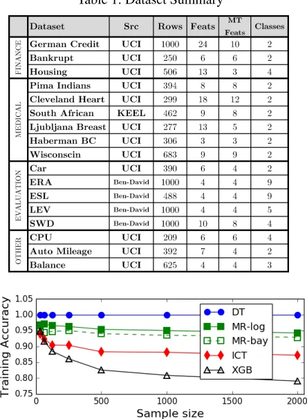
Table 1: Dataset Summary

Figure 5: Training acc of globally MT trees (simulated data).

The NB assumption is false because the rules are condi-tionallydependent, so the predicted probabilities unreliable (pushed to 0 or 1). Nonetheless the surprisingly good perfor-mance of NB is well known (Rish 2001) and worth consid-ering given the computational advantage.

So far we have created a monotone binary Random For-est. For multi-class ordinal applications we use Kotlowski monotone ensembling as described above for PM-RF.

Simulation

To assess the monotonisation loss associated with the glob-ally monotone trees, a simulated dataset was created:

f(x,z)=sign(a0+a1x1+a2x2+a3x3)

where a1, a2, a3 ∈ [0.0,1.0] were uniform random, a0 was chosen to give 50:50 class balance, training data x1, x2, x3, z1, z2, z3 ∈ [−1.0,1.0] were uniform random, sample sizes between 32 and 2000 and 100 experiments. Noise was introduced by reversing 5% of the class labels. Trees were built to leaf purity withmtryof2.

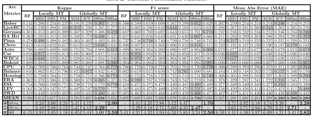
Table 2: Classifier Performance Measures

Figure 6: Classifier Nonmonotonicity for local approaches. M N C is proportion of test points with nonmonotone pre-dictions, for least monotone feature (M N Cmax).

Datasets and Experiments

Datasets.The 17 datasets in Table 1 were used, from UCI (Lichman 2013) and KEEL (Alcala et al. 2010). Missing value rows were removed.

Experiment Design. 100 experiments were performed, with 2₃ of data randomly selected for training and the re-mainder as test. Sub-sampling was stratified and the same partitions were used for all classifiers. Monotone features were identified from domain knowledge. 200 unpruned trees were used in each ensemble. The optimal mtry was

esti-mated from minimumout-of-bagmisclassification rate on a parameter sweep ofmtry ∈ {1,2,3,4,5,6,8,10,12,14}.

Measurement of Ordinal Classifier Accuracy.For ordi-nal classification on imbalanced data, we want to account forerror distance(i.e. for class 4 a prediction of 1 is worse than 3) and class imbalance (so as not to reward random agreement). An ideal measure that accounts for both is lin-ear weighted Cohen’s Kappa(Ben-David 2008). We also re-port Mean Absolute Error (MAE) (which accounts for error distance but not random agreement) and F-measure (which accounts for class imbalance but not error distance).

Results and Discussion

MonotonicityFigure 6 shows that the local techniques generally have non-zero monotonicity noncompliance.

Gen-Table 3: Adjusted P-values for Rank Differences (Hommel)

erally FSD-RF is best (median M N Cmax = 0.9%),

fol-lowed by PM-RF (1.6%) and MID-RF (1.8%). The out-lier for FSD-RF and MID-RF is the ERA dataset, where M N Cmax≥15%! PM-RF is better withM N Cmax=5.2%.

ERA is a highly non-monotone dataset. Thus local ap-proaches can retain significant non-monotonicity.

AccuracyWe first test our hypothesis that MR-RF can achieve lower loss monotonisation and higher accuracy. Ex-amining Table 2, both MR-RF variants achieve the best rank and mean for all metrics. Statistically we follow Demsar (2006) and use non-parametric rank tests. The Friedman test for equal rank is rejected at α = 0.05(Fcrit = 2.33)

withχ2

F of 32.4, 33.9, and 16.0 for MR-RF-log in Kappa,

F-measure and MAE, and 29.7, 23.4 and 13.4 for MR-RF-bay. Proceeding with the Hommel test the adjusted p-values are in Table 3. Both are significantly better than the two globally monotone approaches (p 0.05) except ICT-RF in MAE (p = 0.169 for MR-RF-log and p = 0.714 for MR-RF-bay). Compared to the localapproaches MR-RF-log achieved close to a significant difference for all (pnear

0.10) except PM-RF in MAE (p = 0.169), while MR-RF-bay is insignificantly different for all (p >0.3). Thus MR-RF-log is the stronger of the two, but MR-RF-bay neverthe-less performs very well. Altogether we have strong support for our thesis, albeit imperfect.

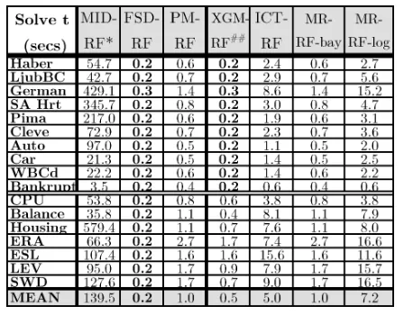
Table 4: Classifier Solve Times. * MID-RF is pure python. ## XGM-RF estimated as(C-1)×FSD-RF.

0.017 and 0.025. These are notable improvements given the impressive performance of standard RF.

Complexity Computation times are in Table 4. Apart from XGM-RF and MID-RF, the techniques have compara-ble implementations based onscikit-learn’s Decision-TreeClassifier, withcythonoptimisations for array opera-tions. XGM-RF and MID-RF were pure python and thus at a significant disadvantage. For XGM-RF it was possible to estimate comparable times by multiplying the FSD-RF time by(C−1). For MID-RF no obvious correction was possible and times should be regarded lightly.

To solve the constrained logistic regression for MR-RF-log we use Newton Conjugate Gradient (scipy’s

fmin-tnc) although many gradient or Newton methods can be used. Complexity can be difficult to estimate for gradient methods but worst case isO( ˜N2.5_{)(Shewchuk et} al. 1994). This is solvedC−1 times per tree, resulting in O(ntreeCN˜2.5). MR-RF-bay isO(ntreeCpN˜2), but in

con-trast is closed form, making it highly competitive.

Conclusions and Future Work

This paper compiled the state-of-the-art monotone tree en-semble approaches from both the literature and popular li-braries, critiqued their mechanisms, and proposed a lower loss (bias) monotonisation method that works better with the variance reducing mechanism of Random Forest.

The proposed MR-RF-log increased experimental accu-racy with globally guaranteed monotonicity and reasonable solution times. The approximate MR-RF-bay was slightly weaker, but still dominated the existing approaches and did so with a very fast closed form solution. Thelocal meth-ods had measureable nonmonotonicity, supporting the value of global monotonicity. Compared to standard RF, improve-ments in all metrics were seen, supporting the value of monotone knowledge purely for the sake of accuracy.

Future work includes developing a bespoke MR-RF-log solver, and automated monotone feature selection.

References

Alcala, J.; Fernandez, A.; Luengo, J.; Derrac, J.; Garcia, S.; Sanchez, L.; and Herrera, F. 2010. Keel data-mining soft-ware tool: Data set repository. Journal of Multiple-Valued Logic and Soft Computing17(255-287):11.

Bartley, C.; Liu, W.; and Reynolds, M. 2016. A novel tech-nique for integrating monotone domain knowledge into the random forest classifier. In Fourteenth Australasian Data Mining Conference (AusDM 2016), volume 170 ofCRPIT. Canberra, Australia: ACS.

Ben-David, A. 1995. Monotonicity maintenance in information-theoretic machine learning algorithms. Ma-chine Learning19(1):29–43.

Ben-David, A. 2008. Comparison of classification accuracy using cohen’s weighted kappa. Expert Systems with Appli-cations34(2):825–832.

Bonakdarpour, M.; Chatterjee, S.; Barber, R. F.; and Laf-ferty, J. 2018. Prediction rule reshaping. arXiv preprint arXiv:1805.06439.

Breiman, L. 2001. Random forests. Machine learning 45(1):5–32.

Chen, T., and Guestrin, C. 2016. Xgboost: A scalable tree boosting system. InProceedings of the 22nd ACM SIGKDD Int’l Conf on Know. Disc. and Data Mining, 785–794. ACM. Demsar, J. 2006. Statistical comparisons of classifiers over multiple data sets. The Journal of Machine Learning Re-search7:1–30.

Fernandez-Delgado, M.; Cernadas, E.; Barro, S.; and Amorim, D. 2014. Do we need hundreds of classifiers to solve real world classification problems? The Jnl of Ma-chine Learning Research15(1):3133–3181.

Gonz´alez, S.; Herrera, F.; and Garcia, S. 2015. Monotonic random forest with an ensemble pruning mechanism based on the degree of monotonicity. New Generation Computing 33(4):367–388.

Hastie, T.; Tibshirani, R.; and J., F. 2009. The Elements of Statistical Learning. Springer.

Kotlowski, W. 2008. Statistical approach to ordinal classi-fication with monotonicity constraints. Ph.D. Dissertation, Poznan University of Technology Institute of Computing Science.

Lichman, M. 2013. Uci machine learning repository. Rish, I. 2001. An empirical study of the naive bayes classi-fier. InIJCAI 2001 workshop on empirical methods in arti-ficial intelligence, volume 3, 41–46. IBM.

Shewchuk, J. R., et al. 1994. An introduction to the conju-gate gradient method without the agonizing pain.

van de Kamp, R.; Feelders, A.; and Barile, N. 2009. Isotonic classification trees. Advances in Intelligent Data Analysis VIII405–416.