Forestry & Natural-Resource Sciences Last Correction: Apr. 4, 2017
USING SATSCAN
TMSPATIAL-SCAN SOFTWARE WITH
NATIONAL FOREST INVENTORY DATA: A CASE STUDY IN
SOUTH CAROLINA
KaDonna Randolph
USDA Forest Service, Southern Research Station, Knoxville, TN 37919 USA
Abstract.The USDA Forest Service Forest Inventory and Analysis (FIA) program makes and keeps
current an inventory of all forest land in the United States. To comply with privacy laws while at the same time offering its data to the public, FIA makes approximate plot locations available through a process known as perturbing (“fuzzing”) and swapping. The free spatial scanning software program SaTScanTM
together with FIA data was used to examine the effects of this process and other arrangements of FIA data on the detection of hotspots of standing dead trees in South Carolina. Only 77.8%, 85.7%, and 66.7% of the hotspots identified in datasets with unaltered plot coordinates were observed when the coordinates were fuzzed, swapped, or both fuzzed and swapped, respectively. Aggregating plot-level data to census tract and county dampened the effect of fuzzing and swapping but resulted in the identification of fewer hotspots overall. Within the framework of forest health monitoring in which failing to identify a problem that truly exists can have serious repercussions, neither relying solely on fuzzed and swapped data nor aggregated data will suffice. The addition of buffer data to evaluate the stability of hotspots located near the study area boundary is recommended.
Keywords: FIA data, hotspot detection, point pattern analysis, SaTScanTM, spatial scan statistic.
1
introduction
Spatial scan statistics are commonly used in epidemi-ology, criminepidemi-ology, and other fields to identify areas with an outbreak of disease, crime, or other unusual event commonly known as a “hotspot.” Hotspot detection re-lies on spatially-referenced point data and an algorithm that scans a geographical area and tests via a likelihood ratio whether the points inside the scanning window (usu-ally a circle or ellipse) have a higher (or lower) rate of event occurrences than the points outside the scanning window. In addition to the underlying distribution of the phenomenon being investigated, the ability of spatial scan statistics to detect hotspots is dependent upon the location accuracy of the spatially-referenced point data and other input required by the scanning algorithm.
Spatial scan statistics have found recent, albeit some-what limited, application to forestry, e.g., having been used to identify hotspots of forest fires (Orozco et al. 2012), oak regeneration (Fei 2010), forest fragmentation (Coul-ston and Riitters 2003, Riitters and Coul(Coul-ston 2005), insect and pathogen disturbances (Coulston and
Riit-ters 2003), and poor tree crown conditions (Bechtold and Coulston 2005). Unique among these applications were the studies by Bechtold and Coulston (2005) and Coulston and Riitters (2003) which employed the spatial scan statistic within the tiered forest health monitoring framework of the U.S. Forest Service (Riitters and Tkacz 2004). This framework consists of a detection tier, which is the routine and repeated, systematic sampling of the forest, and an evaluation tier which provides for intensive follow-up studies of irregularities observed in the detec-tion tier. Together these activities seek to identify the extent and cause of deteriorating forest conditions that are occurring either subtly over a long period of time due to cumulative stresses or more rapidly due to specific stresses (Riitters and Tkacz 2004).
Ground surveys conducted by the Forest Inventory and Analysis (FIA) program of the Forest Service, U.S. Department of Agriculture, are a major source of data for forest health monitoring efforts in the United States. FIA has been conducting a forest inventory in the United States for over 80 years (USDA Forest Service 1992). Established initially by the McSweeney-McNary Forest
Copyright©2017 Publisher of theMathematical and Computational Forestry & Natural-Resource Sciences
Research Act of 1928 (P.L. 70-466), the 1998 Agricul-tural Research, Extension, and Education Reform Act
(P.L. 105-185) mandated FIA to annually report on
the area of forestland; volume, growth, and removal of forest resources; and the health and condition of the resource across all lands, public and private (McRoberts et al. 2005, USDA Forest Service 1992). In addition to these annual reports, which are made available in both print and electronic formats, FIA also makes its raw inventory data available to the public. Standard inventory data such as tree height and diameter, forest type, stand age, etc., as well as information needed to make population estimates, are provided via the online FIA database accessible at http://apps.fs.fed.us/fiadb-downloads/datamart.html [Date accessed: February 26, 2016] (O’Connell et al. 2014).
Despite the plethora of data available through the online database, FIA is restricted from releasing exact plot locations by the 2000 Interior and Related Agencies Appropriations Act (H.R. 3423). To comply with this policy while at the same time offering its data to the public, FIA makes approximate plot locations available through a process known as perturbing and swapping (McRoberts et al. 2005). This process, also called “fuzzing and swapping,” perturbs the geographic coordinates of each plot location to within 1.6 km of its exact location and for a small proportion of the privately owned plots, exchanges the coordinates with other ecologically similar plots in close proximity (McRoberts et al. 2005). Except in unusual circumstances, coordinates are fuzzed and swapped within the same county or parish.
Several studies have examined the effect of fuzzing and swapping on the outcomes of different research questions and have shown that the process has varying effects. For example, studies that use FIA plot data in conjunction with satellite imagery or other spatially explicit data, e.g., digital terrain data, are affected most (Coulston et al. 2006, Prisley et al. 2009, Randolph 2015, Wang et al. 2011), whereas the effect is typically negligible for studies making estimates or building models for large areas (Gibson et al. 2014, Guldin et al. 2006, McRoberts et al. 2005, Prisley et al. 2009). Although many questions regarding the effect of fuzzing and swapping have been answered, questions continue to arise as new technologies are developed and used in conjunction with FIA data. Such is the case with spatial scan statistics. Thus, the objective of this study was to examine the effect of using various arrangements of FIA data to detect hotspots of standing dead trees in South Carolina with the free spatial scanning software program SaTScan1(Kulldorff
and Information Management Services, Inc. 2015). The
1SaTScanTM is a trademark of Martin Kulldorff. The
SaTScanTMsoftware was developed under the joint auspices of
(i) Martin Kulldorff, (ii) the National Cancer Institute, and (iii)
first evaluation examines the effect of fuzzing, swapping, and fuzzing and swapping combined on the size, number, and location of hotspots of standing dead trees in South Carolina (Section 4). The second evaluation examines the effect of aggregating plot data to larger administrative units (census tract and county) as a way to minimize the effect of fuzzing and swapping (Section 5). Because edge effect, or boundary bias, is a concern for spatial analyses like hotspot detection (Gregorio et al. 2006, Van Meter et al. 2010), the third evaluation examines the stability of hotspots detected near the boundary of the study area (Section 6).
2
Spatial Scan
Hotspot detection was implemented with SaTScanTM version 9.4.2 (Kulldorff 2015, Kulldorff and Information Management Services, Inc. 2015). SaTScan works by imposing a scanning window of increasing size at each geographic point of data and testing via a likelihood ratio whether the points inside the scanning window have a higher (or lower) rate of event occurrences, i.e., cases, than the points outside the scanning window (Kulldorff 1997). The maximum size of the scanning window can be a percentage of the population at risk or a defined geographic distance. (The default setting is 50% of the population at risk.) For each scanning window, a likeli-hood ratio test statistic (LRTS) is calculated according to a specified probability model and the window corre-sponding to the maximum value of the calculated LRTS is identified as the most likely hotspot. Other hotspots follow in rank order according to the LRTS. Statistical significance of the hotspots is determined by Monte Carlo simulation that repeats the analysis for a user-specified number of random replications of the original data set under the null hypothesis of spatial randomness. (The default number of replications is 999.) The LRTSs for the hotspots are compared to the distribution of test statistics from the Monte Carlo simulation and if they exceed 95% of the values from the simulation they are considered significant at the 5% level.
For all analyses in this study, the null hypothesis was that the prevalence of standing dead trees in the scanning window was the same as the prevalence of standing dead trees outside the window, i.e., spatial randomness. The alternative hypothesis was that the prevalence of stand-ing dead trees in the window was greater than expected under the null hypothesis. All runs of SaTScan were implemented as purely spatial scans under the Bernoulli probability model with a circular scanning window. The maximum size of the scanning window was defined as a percentage of the total population at risk, i.e., the
combined total of standing dead and live trees (“cases” and “non-cases”, respectively) in the study area, and the number of replications for the Monte Carlo simulations was set to the default value. Only hotspots that were sig-nificant (α = 0.05) and not geographically overlapped by hotspots with higher LRTS values are discussed in the results. In all analyses, emphasis was placed on the difference between hotspots identified in two contrasting datasets rather than on the veracity of hotspots identified in any particular dataset.
3
FIA Data
FIA plots are located across the United States in such a way that the sampling intensity is 1 plot per approximately 2,400 ha. The sampling frame used to locate each plot on the ground is based on a hexagonal tessellation of the United States with 1 plot randomly located within each hexagon (Reams et al. 2005). Each plot consists of four 7.32 m fixed-radius subplots on which trees≥12.7 cm in diameter at breast height (d.b.h.) are measured. The cluster of subplots is arranged with 1 central subplot and 3 other subplots located 36.6 m from the central subplot at azimuths of 0, 120, and 240 degrees. Each plot is permanently monumented, georeferenced, and measured on a repeating cycle of between 5 and 10 years. All plots within a state are divided into spatially balanced “panels.” A single panel of plots is measured every year so that each state is completely measured once every 5 to 10 years on an ongoing basis. Although measurements are spread over multiple years, the inventories are dated with the year of the most recently collected panel of data. For this analysis, FIA data for inventory year 2012 were obtained from the FIA database for Georgia, North Carolina, and South Carolina (Fig. 1). Only fully forested plots with live or standing dead trees ≥12.7 cm d.b.h. were kept for the analyses (Table 1). According to FIA definitions, the bole of a dead tree must be at least 1.37 m in length
Table 1: Number of live and standing dead trees observed on fully forested plots in select buffer zones surrounding South Carolina (SC).
Geographic area Plots Trees
Live Dead Total
SC only 1,742 46,473 1,899 48,372
SC+6 km buffer 1,866 49,869 2,085 51,954 SC+12 km buffer 1,967 52,670 2,217 54,887 SC+18 km buffer 2,079 55,644 2,386 58,030 SC+neighboring
states∗
7,510 196,065 9,228 205,293
∗Georgia and North Carolina.
and lean less than 45 degrees from vertical in order for it to qualify as “standing dead” (USDA Forest Service 2012). Data from Georgia and North Carolina were only included in the evaluation of edge effect (Section 6).
NC
SC
GA
Figure 1: Location of forest and woody wetlands land cover (Homer et al. 2015) in the states of Georgia (GA), North Carolina (NC), and South Carolina (SC) in the southeastern United States.
4
Fuzzing and Swapping
Three datasets were compiled in order to evaluate the effect of FIA’s fuzzing and swapping procedure on the detection of hotspots of standing dead trees in South Carolina. First was a dataset in which all of the plot locations were the confidential geographic coordinates with no fuzzing and no swapping (hereafter referred to as “actual”). Second was a dataset in which the geo-graphic coordinates were fuzzed but none were swapped (“fuzzed/nonswapped”). Third was a dataset like that available to the public in which all of the geographic co-ordinates were fuzzed and some were swapped (“fuzzed/ swapped”). Among the plots used in this analysis, 18.5% had swapped geographic coordinates. For the scans in this analysis, the maximum size of the scanning window was set to 50% of the population at risk in South Carolina (Table 1).
hotspot to the most distant plot included in the hotspot. Results were compared in a pairwise fashion:
Actual vs. fuzzed/nonswapped, to observe the effect of fuzzing.
Fuzzed/nonswapped vs. fuzzed/swapped, to ob-serve the effect of swapping.
Actual vs. fuzzed/swapped, to observe the effect of fuzzing and swapping combined.
For each pairwise comparison, geographically overlapping hotspot pairs were compared with an intersection-to-union area ratio (Ra) calculated as
Ra= |X
T Y| |XSY|×100
where X and Y represent the km2area of two
geographi-cally overlapping hotspots. Maximum Ra, i.e., Ra =
1, occurs when overlapping clusters have identical center points and equal radii. Ra decreases from the maximum
value and asymptotically approaches 0 as overlapping clusters diverge from one another in terms of size (ra-dius) and/or center point location. Area calculations were made in ArcMapTM 10.3.1 (©ESRI 2015) under the Albers Equal Area Conic projection for North Amer-ica. For some hotspots, the circular area extended beyond the border of South Carolina. In such cases, only the area within South Carolina was included in the Ra
calcu-lation. Ra was not calculated when one of the hotspots
in an overlapping pair consisted of a single plot. The sensitivity of the scan to detect “true” hotspots was calculated as the percentage of hotspots detected in the base dataset also detected in the contrasting dataset. For the examination of the effect of fuzzing and the effect of fuzzing and swapping combined, the base dataset was the actual dataset. For the examination of the effect of swapping, the base dataset was the fuzzed/nonswapped dataset.
4.2 Results A total of 9 different regions, labeled A through I in Fig. 2, were identified as having hotspots of standing dead trees, but only regions A, C, D, E, G, and H were identified in all three datasets. Hotspots were identi-fied in region B with the actual and fuzzed/nonswapped datasets, but not the fuzzed/swapped dataset. Hotspots were identified in regions F and I with the actual dataset only. Hotspots in regions C, D, E, and G were single-plot hotspots in each of the three datasets. The hotspots located in region A were the most likely hotspots in each dataset.
4.2.1 Effect of Fuzzing The scan based on the fuzzed /nonswapped dataset identified 2 fewer hotspots than the
A
B
C E
D
G H
I F
Actual
Fuzzed/nonswapped
Multiplot Single plot Fuzzed/swapped
Figure 2: Hotspots of standing dead trees in South Carolina based on actual, fuzzed/nonswapped, and fuzzed/swapped plot coordinates. Single-plot locations are approximate. The letter A identifies the region with the most likely hotspot. The distance between single-plot locations within hotspot regions C, D, E, and G are exaggerated for visualization purposes.
scan based on the actual dataset (sensitivity = 77.8%), but had no effect on the total number of single-plot hotspots (Fig. 2). Located in region A (Fig. 2), the most likely hotspot in the fuzzed/nonswapped dataset (LRTS = 51.8) included 386 cases across 218 plots (Table 2) and compared favorably to the most likely hotspot in the actual dataset (Ra = 0.98) (Table 3). Hotspots in
regions C, D, E, and G (Fig. 2) were identical in terms of LRTS rank and plot composition, but their locations varied slightly due to the fuzzing procedure. Hotspots in regions B and H (Fig. 2) were also identical in terms of LRTS rank and plot composition, but were different in terms of location and area (Ra = 0.96 and 0.91,
respectively) (Table 3).
4.2.2 Effect of Swapping The scan based on the fuzzed/swapped dataset identified 1 less hotspot than the scan based on the fuzzed/nonswapped dataset (sensitivity = 85.7%), but had no effect on the total number of single-plot hotspots (Fig. 2). Located in region A (Fig. 2), the most likely hotspot in the fuzzed/swapped dataset (LRTS = 51.8) included 611 cases across 382 plots (Table 2) and compared moderately to the most likely hotspot in the fuzzed/nonswapped dataset (Ra = 0.66) (Table 3).
Hotspots in regions C, D, E, and G (Fig. 2) were identi-cally located. Though located in the same general region H, the hotspot identified in the fuzzed/swapped dataset varied considerably in terms of geographic area from the one identified in the fuzzed/nonswapped dataset (Ra =
Table 2: Descriptive statistics for selected hotspots of standing dead trees in South Carolina based on plot data with actual geographic coordinates, fuzzed/nonswapped geographic coordinates, and fuzzed/swapped geographic coordinates. A case is defined as a standing dead tree.
Coordinates Hotspot∗ Number of plots LRTS† Number of cases Radius (km)
Actual A 224 53.1 396 95
Actual B 6 10.8 14 14
Actual H 2 11.2 16 4
Fuzzed/nonswapped A 218 51.8 386 94
Fuzzed/nonswapped H 2 11.2 16 4
Fuzzed/swapped A 382 51.8 611 115
Fuzzed/swapped H 5 13.3 16 9
∗Illustrated in Fig. 2.
†Likelihood ratio test statistic.
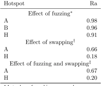
Table 3: Intersection-to-union ratio (Ra) of the geograph-ically overlapping multiplot hotspots illustrated in Fig. 2.
Hotspot Ra
Effect of fuzzing∗
A 0.98
B 0.96
H 0.91
Effect of swapping†
A 0.66
H 0.18
Effect of fuzzing and swapping‡
A 0.67
H 0.20
∗Actual vs. fuzzed/nonswapped.
†Fuzzed/nonswapped vs. fuzzed/swapped.
‡Actual vs. fuzzed/swapped.
4.2.3 Effect of Fuzzing and Swapping Combined
The scan based on the fuzzed/swapped dataset identi-fied 3 fewer hotspots than the scan based on the actual dataset (sensitivity = 66.7%), but had no effect on the total number of single-plot hotspots (Fig. 2). Located in region A (Fig. 2), the most likely hotspot in the actual dataset (LRTS = 53.1) included 396 cases across 224 plots (Table 2) and compared moderately to the most likely hotspot in the fuzzed/swapped dataset (Ra =
0.67) (Table 3). The single-plot hotspots in regions C, D, E, and G (Fig. 2) were identical in terms of plot com-position, but their locations varied slightly due to the fuzzing procedure. Though located in the same general region H, the hotspot identified in the actual dataset varied considerably in terms of geographic area from the one identified in the fuzzed/swapped dataset (Ra =
0.20) (Table 3).
4.3 Discussion The FIA process of fuzzing and swap-ping plot geographic coordinates provided to the public is necessary for protecting landowner privacy. From the outset, it was determined that the act of fuzzing alone was not sufficient to meet the confidentiality requirements required by law (Guldin et al. 2006). Thus, the second step of exchanging the coordinates of ecologically similar plots was added. The decision to add swapping in order to improve confidentiality was evident in this study, for fuzzing alone only minimally effected the spatial scan outcome. That is, the geographic location of individual hotspots identified in the actual dataset was much more similar to hotspots identified in the fuzzed/nonswapped dataset than to hotspots identified in the fuzzed/swapped dataset (Ra >0.90 vs. Ra<0.68).
As observed in other studies (Coulston et al. 2006, Prisley et al. 2009, Wang et al. 2011), using the publicly available FIA data, i.e., fuzzed/swapped data, carries with it risks that may be unacceptable for certain inves-tigations. Typically within the forest health monitoring framework, a high rate of false positives is accepted as the cost of not overlooking a serious problem (Riitters and Tkacz 2004). Accepting such is particularly war-ranted when resources are available to investigate and either confirm or nullify a suspected hotspot (e.g., Bech-told and Coulston 2005, Randolph et al. 2009). No false positives were identified in the fuzzed/swapped dataset; however, there were 3 false negatives. Though this was a moderate rate of success, failing to identify a forest health problem when one actually exists can have serious repercussions. Thus, if the goal is to identify all possible hotspots for further investigation, using fuzzed/swapped data with SaTScan would not suffice.
5
Data Aggregation
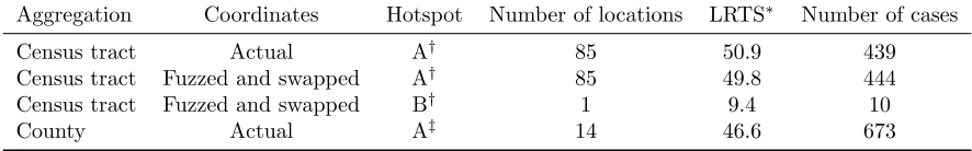
Table 4: Descriptive statistics for hotspots of standing dead trees in South Carolina based on census tract and county aggregations of individual plot data. A case is defined as a standing dead tree.
Aggregation Coordinates Hotspot Number of locations LRTS∗ Number of cases
Census tract Actual A† 85 50.9 439
Census tract Fuzzed and swapped A† 85 49.8 444
Census tract Fuzzed and swapped B† 1 9.4 10
County Actual A‡ 14 46.6 673
∗Likelihood ratio test statistic.
†Illustrated in Fig. 6.
‡Illustrated in Fig. 5.
concerns about plot confidentiality; however, as seen in the field of human epidemiology, aggregating data to administrative units such as county, zip code, or census tract can negatively affect hotspot detection rates (Jeffrey et al. 2009, Olson et al. 2006, Ozonoff et al. 2007). This is because data aggregation can incongruently alter the concentration of events or cases relative to background population levels. This is particularly the case when a hotspot crosses the artificial, administrative boundary by which the aggregations are defined. Though FIA makes every effort to work with partners wishing to use actual geographic coordinates in analyses that require them2,
such requests take time to be approved and fulfilled. Data aggregation might be an alternative to using actual plot coordinates for spatial scan applications if hotspots present at the plot-level can be successfully identified within the aggregated data. Thus, this section explores how well hotspots identified at the plot-level are iden-tified at coarser spatial scales and if the same level of agreement can be achieved by basing the aggregations on the fuzzed/swapped dataset as on the actual dataset.
5.1 Analysis Plot-level counts of standing dead trees (cases) and live trees (non-cases) were respectively summed
by census tract and county. The census tract aggregation was completed twice, once with the actual dataset and secondly with the fuzzed/swapped dataset (Section 4). County-level aggregations needed to be done only once because plots were fuzzed and swapped within counties. The respective sums were assigned to the geographic co-ordinates of the census tract centroid or county centroid. Centroids were determined with the calculate geometry function in ArcMapTM 10.3.1 (©ESRI 2015). Spatial scans were implemented with the maximum size of the scanning window set to 50% of the population at risk in South Carolina (Table 1). Results from the scans based
2More information about this type of arrangement can
be obtained by contacting FIA Spatial Data Services
(http://www.fia.fs.fed.us/tools-data/spatial/index.php) [Date ac-cessed: February 1, 2017].
on the aggregated data (actual dataset) were compared visually to the plot-level scan (actual dataset) (Section 4) through a geographic information system (GIS) overlay. Results from the two census-tract aggregations were com-pared to one another with the intersection-to-union area ratio (Ra) (Section 4.1). For this calculation of Ra, the
area of each hotspot equaled the total area of all census tracts included in the hotspot.
5.2 Results
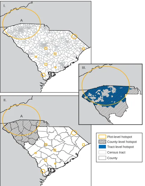
5.2.1 Census tract and county aggregations Only 1 hotspot was identified when the plot-level data (actual dataset) were aggregated to census tract (Fig. 3). This hotspot included 439 cases and 85 census tracts (Ta-ble 4), and excluded tracts roughly corresponding to the Interstate-85 corridor and cities of Greenville and Spar-tanburg. Likewise, only 1 hotspot was identified when the plot-level data were aggregated to county (Fig. 3). This hotspot included 673 cases and 14 counties (Table 4). Both the census tract hotspot and the county hotspot coincided geographically with the most likely hotspot identified in the plot-level data (Fig. 3). The coarser the aggregation, the greater the effect on the detection of hotspots (Ozonoff et al. 2007). Thus, as expected, the extent of the census tract hotspot more closely re-sembled the extent of the plot-level hotspot than did the county-level hotspot. Eight of the 9 hotspot regions identified in the plot-level data were not identified in either aggregated dataset (sensitivity = 11.1%).
ag-I.
II.
III.
A A
Census tract County Plot-level hotspot County-level hotspot Tract-level hotspot
Figure 3: Hotspots of standing dead trees in South Car-olina based on individual plot data (actual coordinates) and plot data (actual coordinates) aggregated to census tract (I) and county (II). Inset (III) highlights the extent of geographical overlap of the plot-, census tract-, and county-level hotspots. Single-plot locations (shown as squares) are approximate. The letter A identifies the region with the most likely hotspot.
Actual Fuzzed/swapped Census tract
B
A
Figure 4: Hotspots of standing dead trees in South Car-olina based on plot data aggregated to census tract using actual geographic coordinates and fuzzed/swapped geo-graphic coordinates. The letter A identifies the region with the most likely hotspot.
gregation to census tract based on the actual dataset is considered to represent true hotspots, then the aggrega-tion based on the fuzzed/swapped dataset resulted in 1 false positive.
5.3 Discussion A high number of false negatives was observed when the scans based on the aggregated data were compared to the scans based on the plot-level data. This occurred at both scales of aggregation, county and census tract, and for both sets of geographic coordinates, actual and fuzzed/swapped. Though one hotspot was consistently identified across all scans, the rate of success was too low to recommend relying solely on aggregated data for forest health monitoring purposes. Nonetheless, aggregating data from precise locations may sometimes be profitable despite the occurrence of false negatives. Jeffrey et al. (2009) showed that the power to detect hotspots was highest with precise locations and disturbances that were confined to small regions of the study areas or those that affected a large portion of the population, but they also observed that aggregation could improve the ability to detect weak signals if the level of aggregation was equal to, or smaller than, the spatial disturbance. Weak signals may represent areas with an emerging problem and could be important with regard to forest health monitoring. Because the distribution of risk is not knowna priori, utilizing multiple levels of aggregations in addition to the precise locations could be beneficial for identifying forest health problems. In so doing, a decision must be made about which plot coordinates to use for aggregations smaller than the county-level. As seen here, the geographical similarity between the census tract aggregations was exceptionally high for the most likely cluster (Ra = 0.96) and a
considerable improvement over what was observed at the plot-level (Ra = 0.67). Nevertheless, the false
positive hotspot reveals the uncertainty that can arise when fuzzing/swapping moves plots from one aggregation unit and into another. Ideally then, aggregations to units smaller than county should be made with actual geographic coordinates.
6
Edge Effect
The second is the inclusion of data from a buffer zone around the area of interest (Bechtold and Coulston 2005, Sadler et al. 2011, Van Meter et al. 2010). The former minimizes the chance that hotspots will reach or extend beyond the boundary of the study area whereas the latter maximizes full estimation of hotspots within the study area.
Choosing a scanning window size that is too large may produce hotspots that are too large to be useful or hide small, homogeneous hotspots within larger, het-erogeneous ones; choosing a size that is too small may produce results that miss large hotspots (Chen et al. 2008, Fotheringham and Zhan 1996). Likewise, an exceedingly large buffer area may alter the overall spatial distribu-tion of risk and unduly influence detecdistribu-tion of hotspots within the interior of the study area. This is especially true if the risk in the buffer area is different from the risk in the area of interest. Two questions that follow from these different approaches, to what size should the scanning window be reduced and what size buffer area is appropriate, are addressed here.
6.1 Analysis An initial, baseline scan was made using the default SaTScan value for the maximum size of the scanning window, i.e., 50% of the total population at risk. Only data from South Carolina (Table 1) were included in the baseline scan. Plot locations were based on the confidential, i.e., actual, geographic coordinates (Section 4).
6.1.1 Scanning window size To address the ques-tion regarding the maximum size of the scanning window, SaTScan was run with maximum scanning window sizes equal to 5%, 15%, 25%, and 33% of the population at risk, i.e., the total number of live and standing dead trees in South Carolina (Table 1). Hotspots identified with these four scanning window sizes were compared to hotspots identified in the baseline scan on the basis of geographical overlap with the intersection-to-union area ratio (Ra) (Section 4.1). Area calculations were made in
ArcMapTM10.3.1 (©ESRI 2015) under the Albers Equal
Area Conic projection for North America. Hotspots were depicted as circles with radii equaling the distance from the plot at the center of the hotspot to the most distant plot included in the hotspot. For some hotspots, the cir-cular area extended beyond the border of South Carolina. In such cases, only the area within South Carolina was included in the Ra calculation. Ra was not calculated
when one of the hotspots in an overlapping pair consisted of a single plot.
6.1.2 Buffer area size To address the question about buffer size, the study area was expanded to include data from 4 buffer areas around South Carolina: (a) within
6-km, (b) within 12-km, (c) within 18-km, and (d) in all neighboring states, i.e., Georgia and North Carolina. The 6-, 12-, and 18-km buffer distances were selected to approximately include the nearest, 2 nearest, and 3 near-est bands of FIA plots, respectively. For these additional scans, the maximum size of the scanning window was set to 50% of the respective population at risk (Table 1). Hotspots identified with each of the scans were compared to hotspots identified in the baseline scan on the basis of geographical overlap with the intersection-to-union area ratio (Ra) (Section 4.1). Hotspots were depicted
as circles with radii equaling the distance from the plot at the center of the hotspot to the most distant plot included in the hotspot. Ra calculations excluded the
area of hotspots extending beyond the South Carolina state boundary and were made only when both hotspots in the overlapping pair consisted of multiple plots.
6.2 Results
6.2.1 Effect of scanning window size The hotspots identified with a maximum scanning window set to 50% of the population at risk were identical to the hotspots identified with a maximum scanning window of 33%, 25%, and 15% of the population at risk. Therefore, only the results for the 5% scanning window are shown in contrast to the results for the 50% scanning window.
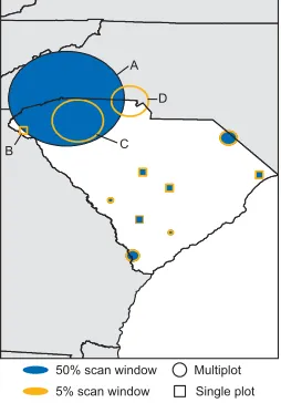
Table 5: Descriptive statistics for selected hotspots of standing dead trees in South Carolina based on a maximum scanning window size of 50% of the population at risk (hotspot A) and 5% of the population at risk (hotspots B, C, and D). A case is defined as a standing dead tree.
Hotspot∗ Number of plots LRTS† Number of cases Radius (km) Ra‡
A 224 53.1 396 95
-B 1 42.3 19 -
-C 85 27.3 153 42 0.43
D 23 18.6 64 30 0.02
∗Illustrated in Fig. 5.
†Likelihood ratio test statistic.
‡Intersection-to-union ratio with hotspot A.
B
50% scan window
5% scan window
Multiplot
Single plot C
D A
Figure 5: Hotspots of standing dead trees in South Car-olina based on two scanning window sizes, 50% of the population at risk and 5% of the population at risk. Single-plot locations are approximate.
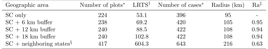
hotspots located in this region increased in area and number of cases as the size of the buffer area increased (Table 6). Similarity between the most likely hotspot in the South Carolina-only scan and the most likely hotspot in the buffer-added scans was approximately the same for buffers of size 6-km, 12-km, and 18-km: Ra = 0.95,
0.94, and 0.94, respectively (Table 6). The similarity between the South Carolina-only scan and the scan with data from South Carolina, Georgia, and North Carolina was lowest of all (Ra = 0.63) (Table 6).
Two hotspots located near the border of South Car-olina, labeled B and C in Fig. 6, were not significant once data in the buffer zones were included in the spatial scan. Hotspot D, located toward the interior of the state, was not detected with buffers>12-km, and hotspots E and F in the interior were not detected when data from Georgia and North Carolina were included (Fig. 6).
IV. III.
II. I.
State State + buffer
Multiplot Single plot A
C F E B
C
B
C D
B
C
D B
D A
A
A
D E E
E
F
F F
Figure 6: Hotspots of standing dead trees in South Car-olina based on data from South CarCar-olina plus data in a buffer area of size 6 km (I), 12 km (II), 18 km (III), and all neighboring states (IV). Single-plot locations are approximate.
Table 6: Descriptive statistics for hotspots in region A (Fig. 6) of South Carolina (SC) based on plot data from select buffer zones. A case is defined as a standing dead tree.
Geographic area Number of plots∗ LRTS† Number of cases∗ Radius (km) Ra‡
SC only 224 53.1 396 95
-SC + 6 km buffer 238 69.2 420 105 0.95
SC + 12 km buffer 240 88.5 422 108 0.94
SC + 18 km buffer 240 102.8 422 108 0.94
SC + neighboring states§ 417 604.3 643 216 0.63
∗Plots and cases outside of SC are excluded.
†Likelihood ratio test statistic.
‡Intersection-to-union ratio with hotspot A identified with the SC-only dataset.
§Georgia and North Carolina.
were deemed unnecessary. Nevertheless, the approach highlighted 3 areas within hotspot A (B, C, and D in Fig. 5) that might be considered core areas and as such could be prioritized for follow-up study. Likewise, the addition of buffer data identified 2 hotspots that are likely artifacts of spatial censoring (B and C in Fig. 6) and could be given low priority in a follow-up study.
A buffer area of 6- to 12-km was sufficient to see changes in the hotspots near the study area boundary. However, whether or not 6- to 12-km should be consid-ered a standard buffer width when using SaTScan to monitor state-level forest health with FIA data was not tested specifically. In general, the size of the buffer area should be chosen carefully, with consideration given to the nature of the resource and disturbance phenomenon under investigation. With FIA’s national sampling frame-work, buffer data are available for all areas except those along the international borders.
Altering the maximum size of the scanning window and adding buffer data are not equivalent forms of evalu-ating edge effects, yet both provide valuable insight into the location and stability of hotspots centered near the boundary of a study area. Subsequently, both tactics may be of use in exploratory analyses such as might be employed within the forest health monitoring framework. It should be noted, however, that selecting hotspots for reporting should not be based on multiple scans uti-lizing different maximum scanning window sizes unless
p-values are adjusted to account for multiple testing (Han et al. 2016).
7
Summary
Detecting hotspots of forest fires, insect and dis-ease outbreaks, or other unusual occurrences within the forested landscape is an essential aspect of monitoring forest health in the same way that detecting outbreaks of human disease is an essential part of monitoring public health. Spatial scan statistics have emerged as a
promis-ing exploratory tool for identifypromis-ing such hotspots at a variety of spatial scales. The utility of these statistics depends upon the location accuracy of the georeferenced forest inventory data and other input required by the scanning algorithms. In this study, SaTScan was used to identify hotspots of standing dead trees in South Car-olina based on national forest inventory data collected by the FIA Program. The effect of three factors on iden-tified hotspots were investigated: the FIA fuzzing and swapping procedure, data aggregation, and edge data.
Overall, this study demonstrated what Gregorio et al. (2006) called the “conditional nature of spatial analy-ses” whereby the size, number, and location of identified hotspots are influenced by the study area size, scanning parameters, and geographical precision of the input data, in addition to the underlying geographic distribution of risk. In all cases, the most likely hotspot of standing dead trees in South Carolina was located in the same general area. Yet it was evident that the FIA process of fuzzing and swapping plot coordinates affected the location, size, and composition of hotspots identified at both the plot and census tract levels. Though aggregating data to cen-sus tract dampened the effect of the fuzzing and swapping procedure, numerous hotspots went undetected when the data were aggregated on the basis of both the actual and fuzzed/swapped geographic coordinates. Hotspots that are detectable at the plot-level but not at the census tract level may be areas of considerable concern if they represent areas where problems are beginning to develop. As such, relying solely on spatial scans based on census tract aggregations is not a suitable practice for forest health monitoring.
ar-eas of the United States or with other variables under different statistical models might produce different con-clusions, particularly regarding the effects of fuzzing and swapping. This is because swapping is only done for privately owned forested plots and between such plots with similar forest characteristics in the same county or parish (Gibson et al. 2014). Thus, the effect of using data with fuzzed/swapped geographic coordinates that was observed in this study may be different in areas with large public land holdings or with variables that are closely tied to the characteristics on which swapping decisions are based, e.g., forest type. In addition, the underlying size of the affected area, i.e., the size of the “true” hotspot, should also be considered. Geographically large hotspots will be less influenced by the swapping procedure than smaller hotspots because the swapping is more likely to occur from within the larger areas than from without (Lister et al. 2005). These factors were not tested directly in this study but could be addressed in a power study using simulated or semisynthetic data in which the distribution of risk is precisely known and controlled (Olson et al. 2006, Ozonoff et al. 2007).
Acknowledgments
I thank Tracey Frescino and Andrew Lister for pro-viding input on an earlier draft of this manuscript. Two anonymous reviewers provided additional input which substantially improved the content of this work. Compar-ing geographically overlappCompar-ing hotspots with the intersec-tion-to-union area ratio was a reviewer suggestion. Fig-ures were formatted according to journal standards with assistance from Janet Griffin.
References
Bechtold, W.A., and J.W. Coulston. 2005. Detection monitoring of crown condition in South Carolina: a case study. IN: McRoberts, R.E., G.A. Reams, P.C. Van Deusen, and W.H. McWilliams eds. Proceedings of the fifth annual Forest Inventory and Analysis sym-posium; 2003 November 18-20; New Orleans, LA. Gen. Tech. Rep. WO-69. Washington, DC: U.S. Department of Agriculture, Forest Service. 222 p.
Chen, J., R.E. Roth, A.T. Naito, E.J. Lengerich, and A.M. MacEachren. 2008. Geovisual analytics to en-hance spatial scan statistic interpretation: an analysis of U.S. cervical cancer mortality. International Journal of Health Geographics. 7:57.
Coulston, J.W., and K.H. Riitters. 2003. Geographic analysis of forest health indicators using spatial scan statistics. Environmental Management. 31(6):764–773.
Coulston, J.W., K.H. Riitters, R.E. McRoberts, G.A. Reams, and W.D. Smith. 2006. True versus perturbed forest inventory plot locations for modeling: a sim-ulation study. Canadian Journal of Forest Research. 36:801–807.
ESRI. 2015. ArcMapTM 10.3.1. Redlands, CA.
Fei, S. 2010. Applying hotspot detection methods in forestry: a case study of chestnut oak regeneration. International Journal of Forestry Research. Article ID 815292.
Fotheringham, A.S., and F.B. Zhan. 1996. A compar-ison of three exploratory methods for cluster detec-tion in spatial point patterns. Geographical Analysis. 28(3):200–218.
Gibson, J., G. Moisen, T. Frescino, and T.C. Edwards, Jr. 2014. Using publicly available forest inventory data in climate-based models of tree species distribution: examining effects of true versus altered location coor-dinates. Ecosystems. 17:43–53.
Gregorio, D.I., H. Samociuk, L. DeChello, and H. Swede. 2006. Effects of study area size on geographic charac-terizations of health events: Prostate cancer incidence in Southern New England, USA, 1994–1998. Interna-tional Journal of Health Geographics. 5:8.
Guldin, R.W., S.L. King, and C.T. Scott. 2006. Vision for the future of FIA: paean to progress, possibilities, and partners. IN: McRoberts, R.E., G.A. Reams, P.C. Van Deusen, and W.H. McWilliams eds. Proceedings of the sixth annual forest inventory and analysis sympo-sium; 2004 September 21–24; Denver, CO. Gen. Tech. Rep. WO-70. Washington, D.C.: U.S. Department of Agriculture, Forest Service. 126 p.
Han, J., L. Zhu, M. Kulldorff, S. Hostovich, D.G. Stinch-comb, Z. Tatalovich, D.R. Lewis, and E.J. Feuer. 2016. Using Gini coefficient to determining optimal cluster reporting sizes for spatial scan statistics. International Journal of Health Geographics. 15:27.
Homer, C.G., J.A. Dewitz, L. Yang, S. Jin, P. Danielson, G. Xian, J. Coulston, N.D. Herold, J.D. Wickham, and K. Megown. 2015. Completion of the 2011 National Land Cover Database for the conterminous United States–representing a decade of land cover change in-formation. Photogrammetric Engineering and Remote Sensing. 81(5):345–354.
Kulldorff, M. 1997. A spatial scan statistic. Communi-cations in Statistics Theory and Methods. 26(6):1481– 1496.
Kulldorff, M. 2015. SaTScanTM user guide for version
9.4. www.satscan.org. [Date accessed: July 6, 2015.]
Kulldorff, M., and Information Management Services, Inc. 2015. SaTScanTM v9.4.2 64-bit: Software for the
spatial and space-time scan statistics. www.satscan.org. [Date accessed: July 6, 2015.]
Lister, A., C. Scott, S. King, M. Hoppus, B. Butler, and D. Griffith. 2005. Strategies for preserving owner pri-vacy in the national information management system of the USDA Forest Service’s Forest Inventory and Analysis Unit. IN: McRoberts, R.E., G.A. Reams, P.C. Van Deusen, W.H. McWilliams, and C.J. Cieszewski eds. Proceedings of the fourth annual forest inventory and analysis symposium; 2002 November 19–21; New Orleans, LA. Gen. Tech. Rep. NC-252. St. Paul, MN: U.S. Department of Agriculture, Forest Service. 257 p.
Loha, E., T.M. Lunde, and B. Lindtjørn. 2012. Ef-fect of bednets and indoor residual spraying on spatio-temporal clustering of malaria in a village in South Ethiopia: A longitudinal study. PLoS ONE. 7(10):e47354.
McRoberts, R.E., G.R. Holden, M.D. Nelson, G.C. Lik-nes, W.K. Moser, A.J. Lister, S.L. King, E.B. LaPoint, J.W. Coulston, W.B. Smith, and G.A. Reams. 2005. Estimating and circumventing the effects of perturb-ing and swappperturb-ing inventory plot locations. Journal of Forestry. 103(6):275–279.
O’Connell, B.M., E.B. LaPoint, J.A. Turner, T. Ridley, S.A. Pugh, A.M. Wilson, K.L. Wad-dell, and B.L. Conkling. 2014. The Forest Inven-tory and Analysis Database: database descrip-tion and user guide for phase 2 (version 6.0.1). U.S. Department of Agriculture, Forest Service. 748 p. www.fia.fs.fed.us/library/database-documentation. [Date accessed: June 25, 2015.]
Olson, K.L., S.J. Grannis, and K.D. Mandl. 2006. Privacy protection versus cluster detection in spatial epidemi-ology. American Journal of Public Health. 96(11):2002– 2008.
Orozco, C.V., M. Tonini, M. Conedera, and M. Kanveski. 2012. Cluster recognition in spatial-temporal sequences: the case of forest fires. Geoinformatica. 16(4):653–673.
Ozonoff, A., C. Jeffery, J. Manjourides, L.F. White, and M. Pagano. 2007. Effect of spatial resolution on cluster detection: a simulation study. International Journal of
Health Geographics. 6:52. DOI 10.1186/1476-072X-6-52.
Perez, A.M., M.C. Thurmond, P.W. Grant, and T.E. Carpenter. 2005. Use of the scan statistic on disaggre-gated province-based data: Foot-and-mouth disease in Iran. Preventive Veterinary Medicine. 71:197–207.
Prisley, S.P., H. Wang, P.J. Radtke, and J. Coulston. 2009. Combining FIA plot data with topographic vari-ables: Are precise locations needed? IN: McWilliams, W., G. Moisen, and R. Czaplewski comps. Forest In-ventory and Analysis (FIA) Symposium 2008; October 21–23; Park City, UT. Proc. RMRS-P-56CD. Fort Collins, CO: U.S. Department of Agriculture Forest Service, Rocky Mountain Research Station. 1 CD.
Randolph, K.C. 2015. Benefits and limitations of us-ing standard Forest Inventory and Analysis data to describe the extent of a catastrophic weather event. e-Res. Pap. SRS-55. Asheville, NC: U.S. Department of Agriculture Forest Service, Southern Research Station. 10 p.
Randolph, K., W. Bechtold, R. Morin, and S. Zarnoch. 2009. From detection monitoring to evaluation moni-toring – a case study involving crown dieback in north-ern white-cedar. IN: McWilliams, W., G. Moisen, and R. Czaplewski comps. Forest Inventory and Analysis (FIA) Symposium 2008; October 21–23; Park City, UT.
Proc. RMRS-P-56CD. Fort Collins, CO: U.S. Depart-ment of Agriculture Forest Service, Rocky Mountain Research Station. 1 CD.
Reams, G.A., W.D. Smith, M.H. Hansen, W.A. Bech-told, F.A. Roesch, and G.G. Moisen. 2005. The For-est Inventory and Analysis sampling frame. p. 11–26 IN: Bechtold, W.A., and P.L. Patterson eds. 2005. The enhanced Forest Inventory and Analysis program— national sampling design and estimation procedures. Gen. Tech. Rep. SRS-80. Asheville, NC: U.S. Depart-ment of Agriculture Forest Service, Southern Research Station. 85 p.
Riitters, K.H., and J.W. Coulston. 2005. Hot spots of perforated forest in the eastern United States. Envi-ronmental Management. 35(4):483–492.
Riitters, K., and B. Tkacz. 2004. Forest health monitor-ing. p. 669–683 IN: Wiersma, B. ed. Environmental Monitoring. Boca Raton, FL: CRC Press.
USDA Forest Service. 1992. Forest Service resource inven-tories: an overview. Washington, D.C.: U.S. Depart-ment of Agriculture, Forest Service, Forest Inventory, Economics, and Recreation Research. 39 p.
USDA Forest Service. 2012. Forest Inventory and Anal-ysis national core field guide. Volume 1: Field data collection procedures for phase 2 plots. Version 6.0. Washington D.C.: U.S. Department of Agriculture Forest Service. 427 p.
Van Meter, E.M., A.B. Lawson, N. Colabianchi, M. Nichols, J. Hibbert, D.E. Porter, and A.D. Liese. 2010. An evaluation of edge effects in nutritional accessi-bility and availaaccessi-bility measures: a simulation study. International Journal of Health Geographics. 9:40.