Water temperature effect on upward air-water flow in a vertical pipe: Local
measurements database using four-sensor conductivity probes and LDA
G. Monrós-Andreu1, S. Chiva1,*, R. Martínez-Cuenca1, S. Torró1, J. E. Juliá1, L. Hernández1 and R. Mondragón1
1
Department of Mechanical Engineering and Construction, Universitat Jaume I, Campus Riu Sec, E-12071, Castellón, Spain.
Abstract. Experimental work was carried out to study the effects of temperature variation in bubbly, bubbly to slug transition. Experiments were carried out in an upward air-water flow configuration. Four sensor conductivity probes and LDA techniques was used together for the measurement of bubble parameters. The aim of this paper is to provide a bubble parameter experimental database using four-sensor conductivity probes and LDA technique for upward air-water flow at different temperatures and also show transition effect in different temperatures under the boiling point.
1 Introduction
Two-phase flows have been studied extensively. These flows can be found in many industrial applications as chemical reactors, nuclear energy production and oil recovery. Many experimental, theoretical and numerical works have been conducted for different pipe sizes, flow rates and fluid properties.
One of the most important key issues in the two-phase flow analysis is the existence of multidimensional interfaces between both phases. The correct behaviour prediction of these interfaces, and its quantification, is
one of the frontieras in the theoretical and experimental
studies of this kind of flow, and up to now, there is not an
effective technique and methodology for the
multidimensional interface characterization in two-phase flow measurement. Then, experimental works play a very important role in the development of new theoretical models and measurement devices.
The basic structure of a two-phase flow can be characterized by three fundamental parameters. These are the void fraction, the Sauter mean diameter (for bubbly flow mainly) and the interfacial area concentration (IAC) [1]. The void fraction expresses the phase distribution and it is a required parameter for the hydrodynamic and thermal design in several industrial processes. The interfacial area concentration describes the available area for the interfacial transfer of mass, momentum and energy, and it is a required parameter for a two-fluid formulation, and the key for most of the industrial applications. The Sauter mean diameter is defined as the diameter of a sphere that has the same volume per surface area ratio as the bubble, and as de interfacial area concentration, is especially important in calculations where the active surface area is important. An accurate knowledge of these parameters is necessary for any two-phase flow analyses.
*
Corresponding author: [email protected]
The use of needle probes as an intrusive method to measure is a well established method for the investigation of multiphase flows. Different measuring techniques can be employed for the needle probes. The most known techniques are based on conductivity, capacitance or optical measurements. Based on the phase identification, these probes can provide information about void fraction, IAC, bubble size, frequency and velocity using simple physical principles.
Measurements of interfacial area in bubbly flow have been done by using double-sensor conductivity probes by Kataoka et al.[2], Hibiki and Ishii [3], Wu and Ishii [4] and Hibiki et al. [5], and four-sensor conductivity probes by Revankar and Ishii [6], Kim, et al. [7]. Furthermore, Hibiki and Ishii [8], Hibiki et al. [9], have developed interfacial area transport equation (IATE), that was formulated by mechanicastically modeling of the physical processes that govern the creation and destruction of interfacial area. At present, more experimental data on interfacial area concentration are needed in order to test the models in modern computerized fluid dynamics (CFD) codes.
The way in which the phases distribute across the pipe have a fundamental influence on important operating parameters such as the friction and heat transfer coefficients. The phase distribution was mapped experimentally by Taitel et al. [10] and different flow regimes were identified such as bubbly, slug, churn and annular. Some experimental correlations have been proposed to predict the transition between flow regimes; however, their dependence on specific flow parameters compromises their general applicability.
It has been observed that for the case of bubbly flows, the bubbles may accumulate preferentially either near the walls (a peak of the gas volume fraction is observed near the wall, i.e., a wall peak) or around the center (a core peak). Serizawa and Kataoka [11] and Zun [12] identified these distinct radial distribution patterns associated to area-averaged void fraction. The pattern classification
This is an Open Access article distributed under the terms of the Creative Commons Attribution License 2 0 , which . permits unrestricted use, distributi and reproduction in any medium, provided the original work is properly cited.
on, EPJ Web of Conferences
DOI: 10.1051/
C
Owned by the authors, published by EDP Sciences, 2013
, epjconf 201/
01105 (2013)
45
34501105
proposed was: wall peak, characterized by a sharp peak of high void fraction near the wall and a ‘valley’ at the channel center with smaller void fraction; and core peak, for which a peak appears around the center of the channel only. The void fraction distribution is correlated with the flow regime as well as some local parameters as interfacial area concentration, gas fraction and superficial velocities. Although there have been some studies that address these issues, S. Méndez-Diaz et al. [13], the mechanisms which determine the phase distribution across the pipe are still partially understood.
A survey of the literature reveals that most investigations of gas/liquid two-phase flow simulation and regime recognition have not considered temperature
effects. The present work aims to establish
experimentally the effect of temperature on the bubble parameters at different temperatures, particularly around transition from bubbly to slug zone, and provide
experimental data for future researches. This
experimental data is obtained with two-phase flow at different axial positions along a vertical pipe using
four-sensor conductivity probes and Laser Doppler
Anemometry (LDA) combined measurements.
The experimental data at different temperatures will help to see how the flow structure changes as the air-water system approaches to transition zone. However, much more information will be needed in order to completely characterize two-phase flow structure at different temperatures.
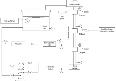
2 Experimental facility
The experimental loop is schematically illustrated in figure. 1. The test section was a round transparent tube made of Plexiglas®, 52mm inner diameter and 5500 mm length. The working fluids in operation were air and water. The water was circulated in the loop by a pair of centrifugal pumps, controlled with a frequency controller device. The air was introduced into the test section through a mixing chamber. Both the flow rates of air and water were measured by flow meters. The bubbles, with diameters ranging from 1 to 3 mm, were generated by a sparger, with an average porosity of 40 microns, located in the base of mixing chamber. Pressure transducers (P0-P4) and temperature sensors (T0-T3) are installed in order to register water and air. The superficial velocity of the liquid phase is measured using a magnetic flow meter (Badger model M100), which provides the superficial velocity of the liquid phase at the inlet of the column test section. Injected air superficial velocity is measured and controlled with a Bronckhorst EL-FLOW flow controller. In order to control water temperature it is necessary to place a heat exchanger (Euroklimat R407C SMART 400/30/50) connected to the water tank so that the system temperature is maintained at a constant temperature in the range between 15 to 37 ° C. Experimental tests are performed at different temperatures, it requires temperature control in the air inlet section (T0) and along the water circuit (T1-T3). In each measurement port pressure sensors are installed (P1-P4) and also before mixing chamber (P0). These sensors have ranges of 0-1 bar to the bottom port, and 0-250mBar for the other two
C
olu
m
n
te
st
s
ec
tio
n
ports.
The interfacial area concentration, void fraction and bubble chord length were measured using four-sensor conductivity probe. The local flow measurements using a four-sensor conductivity probe were carried out at the axial locations of 1166 mm (Low port, L/D=22.4), 3176 mm (Mid port, L/D=61) and 5131 mm (Top port, L/D=98.7).
In order to measure the liquid velocity we use LDA. The LDA equipment consists of a 0.5W Ar+ Ominichrome laser, Dantec Fiberflow beam separator, Dantec FVA 58N40 processor and a PC using the software Floware for data acquisition. The measurements by LDA system were performed at the axial location of 5070 mm (L/D=97.5) from the bottom of the test section.
3 Four sensor conductivity probes
3.1 Methodology
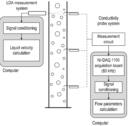
The four-sensor probe measurement system is
schematically shown in figure 2.
Fig 2. LDA and conductivity probe systems
The measurement system consisted of three mounted four-sensor conductivity probes, mechanical traversers, a measurement circuit, a digital high-speed acquisition board, and the software used to signal processing. The four-sensor conductivity probe was attached to the mechanical traverser mounted on a specially designed flange, and it could be moved along the radial direction of the test section using controlled step motors. The measurement circuit was used to measure the potential difference between the exposed tip and the grounded terminal. A high-speed NI SCXI-1000 acquisition board and a PC were used to acquire the voltage signal of the four-sensor probe, with the help of a control program developed under NI LabView software environment. This control program is also used for acquire the data from pressure, temperature and flow transducers and control the centrifugal pumps and air flow controller in order to
prepare a run test. The sampling frequency was set 60 kHz for each conductivity probe, and the sampling time was 30 seconds. Mechanical traverser, is also managed with NI Labview control software in order to move simultaneously and with precision the three conductivity probes through radial positions inside the pipe.
The four- sensor probe is basically a phase identifier. It consists of four sensors made of insulated copper, with a diameter of 0.25 mm. The vertical distance between main and auxiliary tips was about 1.5 mm. The probe is connected to a power supply with a fixed voltage, due to the large difference in conductivity between the liquid phase and the gas phase, the impedance signal acquired rises sharply when a bubble passes through one of the sensor tips.
Fig 3. Four-sensor conductivity probe schema.
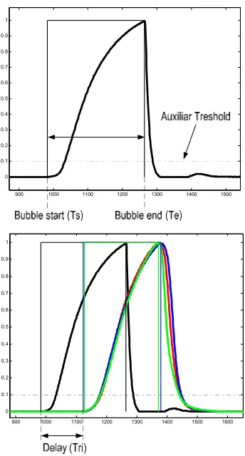
3.2 Signal processing
When the probe sensor is surrounded by liquid, a lower voltage is put out; and when the probe sensor contacts with gas, a higher voltage is obtained. But due to the finite size of each sensor and the time delay needed to wet or rewet the sensor tips, the output signal of the four-sensor probe differed from ideal two-state square-wave. A suitable signal processing technique is therefore necessary to extract the required information from the raw signal. In the present work, processing software in Matlab platform has been developed in order to regenerate the ideal square-wave signal and process it in order to calculate main bubble parameters.
The processing software acts as a phase identifier based on signal level. First the signal is filtered and normalized. After that the code recognizes bubbles start by two different methods: recursive fitting algorithm or direct use of an auxiliary treshold (if the signal noise near rise point is too high for using the recursive fit). Finally,
bubbles ends are computed when signal falls after a relative maximum of the signal.
Signals before and after processing using this method are illustrated in figure 4.
900 1000 1100 1200 1300 1400 1500 1600
0 0.1 0.2 0.3 0.4 0.5 0.6 0.7 0.8 0.9 1
900 1000 1100 1200 1300 1400 1500
0 0.1 0.2 0.3 0.4 0.5 0.6 0.7 0.8 0.9 1
Fig 4. Signal processing.
From the square-wave signal the number of bubbles that hit the sensor can be measured by counting the number of pulses in the signal. The three components of interfacial velocity of each interface can be obtained by using the distance to the different tips of the four-sensor probe, and time delay between the upstream and
downstream signal (Tri) From the local instant
formulation of the two-fluid model, the local time-averaged void fraction can be expressed as the ratio between the accumulated pulse widths of the upward or
downward sensor (Te-Ts) and the total sampling time
during the sampling period.
Local parameters of the two-phase flows can be obtained from two types of information: the residence time of the gas phase in the probe and signal delay recoded between different paired tips. This allows us to record the Chord length, void fraction and average interfacial speed as main parameters directly from acquired data. Once these three parameters are obtained and interfacial area concentration obtained, Sauter mean diameter can be indirectly calculated. The four-sensor conductivity probe method can predict the IAC without any assumptions of bubble shape or interfacial motion for bubbles having a large size relative to the probe.
Delhaye and Bricard [1] pointed out that the structure of a bubbly two-phase flow can be characterized by two
of the three of following parameters: the interfacial area concentration (IAC), the void fraction and the Sauter median diameter. The IAC (a) is defined by the total interface area per unit mixture volume. According to Ishii [14], the local time-averaged IAC at fixed point in space x0 is given by:
( ) = ∑ |
∙ | (2)
Where Ω, l, vil, nil denote the time interval for
averaging, the interface of bubble, the velocity vector of considered interface, the surface normal unit vector of the considered interface at x0 when it passes through x0.
Shen et al., were the first to propose a theoretical proof based on their interfacial measurement theorem for multi-sensor probes, by using vector analysis and pointed out that a four-sensor probe could measure the interfacial velocity component in the interfacial direction. Their methodology enabled the interfacial area concentration measurement and the instantaneous interfacial direction measurement in multi-dimensional two-phase flow. Their expression for the interfacial area concentration measurement is:
a (x ) =
Ω∑ | | (3)
Where Ω is the time interval for averaging, Nt the
total number of interfaces that hit the sensor during the
interval time, and A0, A1, A2, A3 are determinants only
dependant of geometric distribution of the sensor tips and time delay between interfaces.
More details about expression 3 can be found in Shen et al. [15].
Sauter mean diameter (dSM), given by the ratio of the
volume and surface area of a typical bubble, can be calculated as:
d = ∙α (4)
Where α is the void fraction, total gas phase per unit
mixture and a is the interfacial area concentration.
Using the information of processed signal several bubble parameters has been calculated:
Local time-averaged void fraction.
Local time-averaged IAC.
Local Chord length distributions.
Local interfacial velocity.
Local number of bubbles and size based
classification.
Fig 5. Example of interfacial velocity distribution for an axial position. Case jl=0.5 m/s, jg=0.05 m/s, TC, and L/D=61.
For each radial point chord length is calculated as mean value of PDF that fits chord length distribution. For chord length, normal distribution has been considered. Figure 6 shows an example of Chord length distributions for a one axial position.
Fig 6. Example of Chord length distribution for an axial
position. Case jl=0.5 m/s, jg=0.05 m/s, TC and L/D=61.
Detected bubbles are classified depending bubble diameter limit criteria proposed by Ishii et al. [16], using individual bubble interfacial velocity and chord length. Diameter limit for each different type of bubble are:
Table 1. Bubble diameter limit criteria.
Spherical Bubbles Distorted bubbles Cup-slug bubbles 3 / 1 2 4 f N g
Desf
2 / 1 g N f f f g Ddist 4
g DcapMAX 40
3.3 Experimental data
Four-sensor conductivity probes data sets have been taken at different conditions:
Superficial liquid velocities jl: 0.5, 1, 2 m/s.
Superficial gas velocities jg: 0, 0.05, 0.1,
0.15, 0.2, 0.3 m/s.
Temperatures: 15ºC (TC), 21ºC (TA) and
37ºC (TH)
15 radial measurement points at three axial
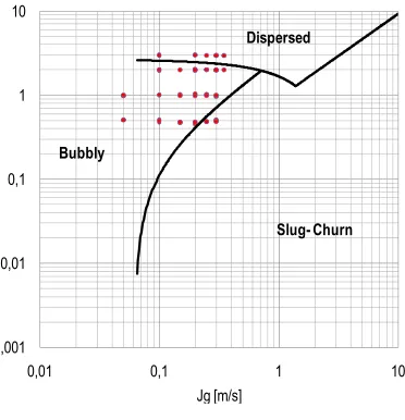
positions (L/D=22.4), L/D=61, L/D=98.7). The flow conditions have been chosen measuring the superficial liquid and air velocity and the average void fraction on L/D=22.4 for each condition. All the conditions (Table 2) are in the bubbly flow regime.
Table 2. Experimental flow conditions for conductivity probes.
Experiments carried out are represented in the flow regime map proposed by Taitel et al [10] shown in figure 7 for a 50 mm pipe inner diameter.
Fig 7. Flow regime map.
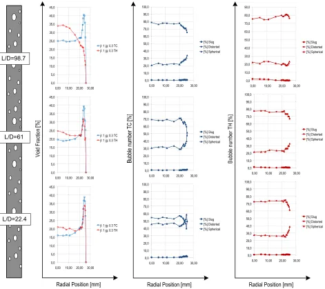
As example of the results obtained using our facility, Figure 8 shows experimental void fraction average
profile data vs radial position for case jl=1 m/s and jg=0.3
at two different temperatures, TC (cool temperature, 15ºC) and TH (hot temperature, 37 ºC). Effect of wall peak to core peak transition and the change in the bubble size radial distribution can be observed.
0 0.5 1 1.5 2 Velocity r00
Velocity [m/s]
0 0.5 1 1.5 2 Velocity r01
Velocity [m/s]
0 0.5 1 1.5 2 Velocity r02
Velocity [m/s]
0 0.5 1 1.5 2 Velocity r03
Velocity [m/s]
0 0.5 1 1.5 2 Velocity r04
Velocity [m/s]
0 0.5 1 1.5 2 Velocity r05
Velocity [m/s]
0 0.5 1 1.5 2
Velocity r06
Velocity [m/s]
0 0.5 1 1.5 2
Velocity r07
Velocity [m/s]
0 0.5 1 1.5 2
Velocity r08
Velocity [m/s]
0 0.5 1 1.5 2
Velocity r09
Velocity [m/s]
Velocity r10 Velocity r11 Velocity r12 Velocity r13 Velocity r14
0 2 4 6
Chord length r00
Chord length [mm] 0 1 2 3 4 5 Chord length r01
Chord length [mm] 0 2 4 6 Chord length r02
Chord length [mm] 0 2 4 6 Chord length r03
Chord length [mm] 0 2 4 6 Chord length r04
Chord length [mm]
0 2 4 6
Chord length r05
Chord length [mm]
0 2 4 6
Chord length r06
Chord length [mm]
0 2 4 6
Chord length r07
Chord length [mm]
0 2 4 6
Chord length r08
Chord length [mm]
0 2 4 6
Chord length r09
Chord length [mm]
0 2 4 6
Chord length r10
Chord length [mm]
0 2 4 6
Chord length r11
Chord length [mm]
0 2 4 6
Chord length r12
Chord length [mm]
0 2 4 6
Chord length r13
Chord length [mm]
0 2 4 6
Chord length r14
Chord length [mm]
Nrun jg [m/s] α [-] T [°C] jg [m/s] α [-] T [°C] jg [m/s] α [-] T [°C]
Run01 0,05 0,06 16,52 Run18 0,05 0,05 15,00 Run35 0,10 0,05 15,87
Run02 0,10 0,13 18,96 Run19 0,10 0,09 14,65 Run36 0,20 0,10 16,27
Run03 0,15 0,19 17,98 Run20 0,15 0,12 14,53 Run37 0,25 0,13 16,57
Run04 0,20 0,24 17,13 Run21 0,20 0,15 14,77 Run38 0,30 0,15 16,79
Run05 0,25 0,28 16,41 Run22 0,25 0,19 14,79 Run39 0,10 0,05 14,78
Run06 0,30 0,32 15,82 Run23 0,30 0,22 15,53 Run40 0,20 0,10 15,34
Run07 0,05 0,06 20,67 Run24 0,05 0,05 23,08 Run41 0,30 0,13 15,75
Run08 0,10 0,13 20,64 Run25 0,10 0,09 23,38 Run42 0,35 0,15 16,06
Run09 0,15 0,19 20,60 Run26 0,20 0,15 24,20 Run43 0,10 0,05 21,33
Run10 0,20 0,24 20,57 Run27 0,25 0,19 24,45 Run44 0,15 0,07 21,60
Run11 0,30 0,31 20,56 Run28 0,30 0,22 23,66 Run45 0,20 0,10 22,64
Run12 0,05 0,07 34,60 Run29 0,05 0,05 35,83 Run46 0,30 0,13 21,42
Run13 0,10 0,13 35,77 Run30 0,10 0,08 36,47 Run47 0,10 0,05 36,56
Run14 0,15 0,20 36,34 Run31 0,15 0,13 36,52 Run48 0,20 0,10 36,68
Run15 0,20 0,25 36,62 Run32 0,20 0,17 36,71 Run49 0,25 0,13 36,55
Run16 0,25 0,27 36,38 Run33 0,25 0,20 36,52 Run50 0,30 0,15 36,46
Run17 0,30 0,27 36,67 Run34 0,30 0,23 36,67 Run51 0,10 0,05 36,54
Run52 0,20 0,10 36,46
Run53 0,25 0,13 36,45
Run54 0,30 0,15 36,79
jl 0.5 m/s jl 1 m/s jl 2 m/s 0,001 0,01 0,1 1 10
0,01 0,1 1 10
The local void fraction profile has a typical evolution of the pressure reduction. The peaks in the void fraction profile were located more or less at one diameter from the wall.
While the evolution of local profile along the pipe at TC maintain the wall peak configuration, same flow configuration at higher temperature TH presents a clear transition or core peak distribution at L/D=98.7.
In TC conditions distorted and spherical are the only bubble size observed, and as the pressure decreases along the pipe it is observed that the percentage of distorted bubbles grows to the detriment of the spherical one mainly due either to the coalescence effect and pressure reduction.
However in TH conditions clearly predominant percentage of distorted bubbles over the spherical. Due to larger size of those bubbles, it tends to move to the center of the pipe changing the void fraction profile to core peak at the top of the pipe. At L/D=98.7 slug bubbles were
clearly detected (2.1 % over total number of bubbles at this radial position)).
It has been observed that a transition or core peak distribution appears when the percentage of slug bubbles computed in the center of the pipe over the total of computed bubbles is greater than 1%.
Figures 9, 10 and 11 show some experimental data results obtained in our facility. Only the extreme values
of jg and jl are shown with the aim to give a clear
representation of the data most important found. General characteristics observed from experimental data:
In the cases without clear core peak
distribution, the cord length is quite uniform.
In all the profiles IAC shows a similar
behaviour of its respective void fraction profile if chord length is more or less uniform
The interfacial velocity has a flat profile for
cases with wall peak distribution.
0,0 5,0 10,0 15,0 20,0 25,0 30,0 35,0 40,0 45,0
0,00 10,00 20,00 30,00
jl: 1 jg: 0.3 TC jl: 1 jg: 0.3 TH
0,0 10,0 20,0 30,0 40,0 50,0 60,0 70,0 80,0 90,0 100,0
0,00 10,00 20,00 30,00 [%] Slug [%] Distorted [%] Spherical
0,0 10,0 20,0 30,0 40,0 50,0 60,0 70,0 80,0 90,0
0,00 10,00 20,00 30,00
[%] Slug [%] Distorted [%] Spherical 0,0
10,0 20,0 30,0 40,0 50,0 60,0 70,0 80,0 90,0 100,0
0,00 10,00 20,00 30,00 [%] Slug [%] Distorted [%] Spherical 0,0
10,0 20,0 30,0 40,0 50,0 60,0 70,0 80,0 90,0 100,0
0,00 10,00 20,00 30,00 [%] Slug [%] Distorted [%] Spherical
0,0 10,0 20,0 30,0 40,0 50,0 60,0 70,0 80,0 90,0 100,0
0,00 10,00 20,00 30,00 [%] Slug [%] Distorted [%] Spherical 0,0
10,0 20,0 30,0 40,0 50,0 60,0 70,0 80,0 90,0 100,0
0,00 10,00 20,00 30,00 [%] Slug [%] Distorted [%] Spherical 0,0
5,0 10,0 15,0 20,0 25,0 30,0 35,0 40,0 45,0
0,00 10,00 20,00 30,00
jl: 1 jg: 0.3 TC jl: 1 jg: 0.3 TH 0,0
5,0 10,0 15,0 20,0 25,0 30,0 35,0 40,0 45,0
0,00 10,00 20,00 30,00
jl: 1 jg: 0.3 TC jl: 1 jg: 0.3 TH
Radial Position [mm] L/D=22.4
L/D=61 L/D=98.7
Radial Position [mm] Radial Position [mm]
Near to the wall, the interfacial velocity decreases due to the wall influence.
With liquid superficial velocity less than 2
m/s and wall peak distribution the increase of
jg has a little influence on the gas velocity
profile and void fraction profile for TC conditions. In some TA and TH cases the
increase of jg may cause the change to a
transition or core peak distribution.
The gas velocity increases substantially
when large bubbles appear in the flow.
Wall peak is located at one bubble diameter
from the wall, but this distance seems to increase slightly with the velocity of the fluid and a greater void fraction.
Hottest liquid produces an increasing of the
magnitude of void fraction in the core peak scenarios.
The bubble size at the top of the pipe
increases with the hottest liquid, then IAC
has reduced values in comparison to the case with coldest liquid.
4. LDA methodology
The Laser Doppler Anemometer, or LDA, is a widely accepted tool for fluid dynamic investigations in gases and liquids and has been used as such for more than three decades. It is a well-established technique that gives information about flow velocity. It is non-intrusive principle and directional sensitivity make it very suitable for applications with reversing flow, chemically reacting or high-temperature media and rotating machinery, where physical sensors are difficult or impossible to use.
LDA measurements have been taken in top port (L/D=97.5), where fully developed flow is achieved.
All experimental data sets with LDA (turbulence intensity and liquid velocity) were realized in the same experimental conditions of corresponding experimental data using conductivity probes.
0,0 5,0 10,0 15,0 20,0 25,0 30,0 35,0 40,0 45,0 50,0
0,00 10,00 20,00 30,00 0,0
5,0 10,0 15,0 20,0 25,0 30,0 35,0 40,0 45,0 50,0
0,00 10,00 20,00 30,00 0,0
5,0 10,0 15,0 20,0 25,0 30,0 35,0 40,0 45,0 50,0
0,00 10,00 20,00 30,00
0,0 0,2 0,4 0,6 0,8 1,0 1,2
0,00 10,00 20,00 30,00
0,0 0,2 0,4 0,6 0,8 1,0 1,2
0,00 10,00 20,00 30,00
0,0 0,2 0,4 0,6 0,8 1,0 1,2
0,00 10,00 20,00 30,00
0,0 1,0 2,0 3,0 4,0 5,0 6,0 7,0 8,0
0,00 10,00 20,00 30,00
0,0 1,0 2,0 3,0 4,0 5,0 6,0 7,0 8,0
0,00 10,00 20,00 30,00
0,0 1,0 2,0 3,0 4,0 5,0 6,0 7,0 8,0
0,00 10,00 20,00 30,00
0,0 100,0 200,0 300,0 400,0 500,0 600,0 700,0 800,0
0,00 10,00 20,00 30,00 0,0
100,0 200,0 300,0 400,0 500,0 600,0 700,0 800,0
0,00 10,00 20,00 30,00 0,0
100,0 200,0 300,0 400,0 500,0 600,0 700,0 800,0
0,00 10,00 20,00 30,00
Fig 9. Void fraction, interfacial velocity, Chord length and IAC for jl=0.5 m/s, jg=0.05-0.3 m/s, 15º(TC), 21ºC (TA) and
37º(TH). The legend is as follows: ( ) jl=0.5 m/s, jg=0.05 m/s, TC; ( ) jl=0.5 m/s, jg=0.3 m/s, TC; ( ) jl=0.5 m/s, jg=0.05 m/s, TA; ( ) jl=0.5 m/s, jg=0.3 m/s, TA; ( ) jl=0.5 m/s, jg=0.05 m/s, TH; ( ) jl=0.5 m/s, jg=0.3 m/s, TH.
The presence of the bubbles leads to increased noise levels compared with LDA in single phase flows. The higher noise levels lead to the occurrence of multiple validations, i.e., the multiple detection of the burst caused by a single particle. This may lead to inaccurate velocity estimates or even outliers. In the processing program the effect was handled by first rejecting velocity realizations with:
| − | > 4 (5)
Being σ the standard deviation of the signal. The next data processing steps are related with the velocity bias correction. In a time varying flow the instantaneous data rate is generally correlated with the instantaneous liquid velocity. As a result, the higher velocities are usually over-represented in the time signal and the velocity moments are biased if simple arithmetic averaging is used (velocity bias). Previous work has shown the importance of velocity bias correction for bubble column flow experiments [17]. The velocity bias correction is
performed by so-called 2D+weighting: inversely
weighing the data with the velocity [18]. Since only two components are known, the magnitude of the third component is estimated from the variance of the second component: the weighting factor is:
=
∙ ′
(6)
With dm/lm as the diameter-to-length ratio of the
ellipsoidal measurement volume, and Vx and Vz as the
lateral and vertical liquid velocity components. The use of only two components is justified since the magnitude of the vertical and lateral fluctuations will be close. Based on the fluctuating component of the velocity, it is possible to define several parameters of interest for the study of turbulence. In particular, the relative turbulence intensity is defined as the ration of the root mean square value of the fluctuation velocity referred to the mean velocity of the flow [19]:
0,0 5,0 10,0 15,0 20,0 25,0 30,0 35,0 40,0 45,0
0,00 10,00 20,00 30,00
0,0 5,0 10,0 15,0 20,0 25,0 30,0 35,0 40,0 45,0
0,00 10,00 20,00 30,00
0,0 5,0 10,0 15,0 20,0 25,0 30,0 35,0 40,0 45,0
0,00 10,00 20,00 30,00
0,0 0,2 0,4 0,6 0,8 1,0 1,2 1,4 1,6 1,8
0,00 10,00 20,00 30,00
0,0 0,2 0,4 0,6 0,8 1,0 1,2 1,4 1,6 1,8
0,00 10,00 20,00 30,00
0,0 0,2 0,4 0,6 0,8 1,0 1,2 1,4 1,6 1,8
0,00 10,00 20,00 30,00
0,0 1,0 2,0 3,0 4,0 5,0 6,0
0,00 10,00 20,00 30,00
0,0 1,0 2,0 3,0 4,0 5,0 6,0
0,00 10,00 20,00 30,00
0,0 1,0 2,0 3,0 4,0 5,0 6,0
0,00 10,00 20,00 30,00
0,0 50,0 100,0 150,0 200,0 250,0 300,0 350,0 400,0 450,0 500,0
0,00 10,00 20,00 30,00 0,0
50,0 100,0 150,0 200,0 250,0 300,0 350,0 400,0 450,0 500,0
0,00 10,00 20,00 30,00 0,0
50,0 100,0 150,0 200,0 250,0 300,0 350,0 400,0 450,0 500,0
0,00 10,00 20,00 30,00
Fig 10. Void fraction, interfacial velocity, Chord length and IAC for jl=1 m/s, jg=0.05-0.3 m/s, 15º(TC), 21ºC (TA) and
37º(TH). The legend is as follows: ( ) jl=1 m/s, jg=0.05 m/s, TC; ( ) jl=1 m/s, jg=0.3 m/s, TC; ( ) jl=1 m/s, jg=0.05
I = ′ =
′ ′ ′
(7)
Where ′ is called the absolute turbulence
intensity.
The turbulence kinetic energy is defined as [20]
k = u′ + u′ + u′ (8)
In order to calculate turbulence intensity we assume
= so with current system we are only able to
measure in two directions, and this two magnitudes will be close.
LDA data acquisition is realized at frequency about 100-300 Hz depending on radial position and until 3000 of samples are acquired.
4.1 Experimental data
In order to obtain a velocity and turbulence profile,
we measure liquid velocity components in axial (y axis)
and radial (x axis) direction with LDA in 15 diameter
pipe radial positions (with and without presence of gas). LDA data sets have been taken at different conditions:
Superficial liquid velocities (jl): 0.5, 1, 2, 3
m/s.
Superficial gas velocities (jg): 0, 0.05, 0.1,
0.15, 0.2, 0.3 m/s.
Temperatures: 15ºC (TC) and 37ºC (TH)
Axial position: L/D=98.7.
Figures 12 and 13 show the liquid velocity profiles obtained with LDA at different temperatures, shown in Table 3.
Table 3. Experimental flow conditions for LDA.
Fig 12. LDA liquid velocity profiles at 15º (TC).
Fig 13. LDA liquid velocity profiles at 37º (TH).
Figures 14 and 15 show turbulence intensity obtained from processed LDA data at different temperatures.
Theoretically we should observe a wall-peak behaviour (turbulence intensity tends to zero near to the wall of the pipe) but due to LDA measurement volume control (above 1-1.5 mm length) we have not enough precision to validate the measurements in that zone near to the wall.
Fig 14. LDA Turbulence intensity profiles at 15º (TC).
jl 0.5 [m/s]
jl 1 [m/s]
Nrun jg [m/s]
α [-]
T [°C] Nrun
jg [m/s]
α [-]
T [°C] RunAA 0.00 0.00 16.12 RunBA 0.00 0.00 16.23
Run01 0.05 0.06 16.52 Run18 0.05 0.05 15.00
Run02 0.10 0.13 18.96 Run19 0.10 0.09 14.65
Run03 0.15 0.19 17.98 Run20 0.15 0.12 14.53
RunAB 0.05 0.07 34.60 Run29 0.05 0.05 35.83
Run15 0.10 0.13 35.77 Run30 0.10 0.08 36.47
Run14 0.15 0.20 36.34 Run31 0.15 0.13 36.52
jl 2 [m/s]
jl 3 [m/s]
Nrun jg [m/s]
α [-]
T [°C] Nrun
jg [m/s]
α [-]
T [°C] RunCA 0.00 0.00 16.03 RunDA 0.00 15.76
Run35 0.10 0.05 15.87 RunDB 0.10 0.05 15.34
Run36 0.20 0.10 16.27 RunDC 0.20 0.10 15.75
RunCB 0.10 0.05 36.56 RunDE 0.10 0.04 36.47
Run48 0.20 0.10 36.68 RunDF 0.20 0.08 36.68
Run49 0.25 0.13 36.55 RunDG 0.30 0.11 36.67
0,0 0,5 1,0 1,5 2,0 2,5 3,0 3,5 4,0 4,5
0 5 10 15 20 25 30
Liq
uid
v
elo
cit
y [
m
/s
]
Radial Position [mm]
RunAA Run01 Run02 Run03 RunBA Run18 Run19
Run20 RunCA Run35 Run36 RunDA RunDB RunDC
0 0,5 1 1,5 2 2,5 3 3,5 4 4,5
0 5 10 15 20 25 30
Liq
uid
v
elo
cit
y [
m
/s]
Radial Position [mm]
RunAB Run15 Run14 Run29 Run30 Run31
RunCB Run48 Run49 RunDE RunDF RunDG
0,0 10,0 20,0 30,0 40,0 50,0 60,0
0 5 10 15 20 25 30
T
ur
bu
le
nc
e i
nte
ns
ity
[%
]
Radial Position [mm]
RunAA Run01 Run02 Run03 RunBA Run18 Run19
Run20 RunCA Run35 Run36 RunDA RunDB RunDC
EPJ Web of Conferences
Fig 15. LDA Turbulence intensity profiles at 15º (TC).
We can observe the effect of increasing gas phase and velocity in zones near to center of the pipe: increasing the amount of gas, turbulence intensity is higher in the center of the pipe due to the alteration caused by the bubbles presence.
Increment of turbulence not seems to be proportional
to the amount of gas: from single phase to jg=0.05 (about
5% of void fraction) the turbulence intensity at the center of the tube increase, but further gas increments seem to increase the turbulence intensity in a more moderate way. For void fractions above 25%, the increase of the gas does not seem to increase the turbulence intensity.
For low liquid velocity, less than 1 m/s, the presence of bubbles seems to decrease the turbulence intensity near the wall. It can be observed in figures 17 and 18.
Fig 16. LDA Turbulence intensity profiles at jl=0.5 m/s, 15º
(TC).
Fig 17. LDA Turbulence intensity profiles at jl=3 m/s, 15º (TC).
Same behaviour is observed for the hot temperatures in Figures 18 and 19, but with few differences: due to lower viscosity of hot water, turbulence intensity profile seems to be more flattened near to the wall.
Fig 18. LDA Turbulence intensity profiles at jl=1 m/s, 37º
(TH).
Fig 19. LDA Turbulence intensity profiles at jl=2 m/s, 37º(TH).
At jl=1 m/s Figure 20 shows how at jl=1 m/s, 5% void
fraction and variation of temperature affect to velocity profile: turbulence intensity caused by bubbles makes velocity profile more flattened near the wall. It can be
0 10 20 30 40 50 60
0 5 10 15 20 25 30
T
ur
bu
le
nc
e i
nte
ns
ity
[%
]
Radial Position [mm]
RunAB Run15 Run14 Run29 Run30 Run31
RunCB Run48 Run49 RunDE RunDF RunDG
0,0 10,0 20,0 30,0 40,0 50,0 60,0
0 5 10 15 20 25 30
T
ur
bu
le
nc
e i
nte
ns
ity
[%
]
Radial Position [mm] jg = 0 m/s
jg = 0,05 m/s jg = 0,1 m/s jg = 0,15 m/s
0,0 10,0 20,0 30,0 40,0 50,0 60,0
0 5 10 15 20 25 30
T
ur
bu
le
nc
e i
nte
ns
ity
[%
]
Radial Position [mm] jg = 0 m/s
jg = 0,1 m/s
jg = 0,2 m/s
0,0 10,0 20,0 30,0 40,0 50,0 60,0
0 5 10 15 20 25 30
T
ur
bu
le
nc
e i
nte
ns
ity
[%
]
Radial Position [mm] jg = 0,05 m/s
jg = 0,1 m/s
jg = 0,15 m/s
0,0 10,0 20,0 30,0 40,0 50,0 60,0
0 5 10 15 20 25 30
T
ur
bu
le
nc
e i
nte
ns
ity
[%
]
Radial Position [mm] jg = 0,1 m/s
jg = 0,2 m/s
jg = 0,25 m/s
observed the major effect of flattened profile at high temperature: in this case the increase is due to combination of less liquid phase density and bubble agitation.
Fig 20. LDA Velocity profiles at jl=1 m/s, jg =0.05 m/s 15º(TC)
and 37º(TH) and jl=1 m/s; jg =0 m/s 15º(TC).
Figure 21 shows a map of the Reynolds and Weber numbers all experimental data considered in this paper. The solid markers show measures at different conditions and different axial point measurement whereas empty markers show either transition or core peak distributions. Only measures which shows core peak distribution in L/D=98.7 are marked, so we can assure fully developed flow in this stage.
Criteria assumed to consider transition or core peak distribution has been the percentage of slug bubbles in the center of the pipe. If slug bubble number is above 1% of the total computed bubbles transition or core peak distribution is considered.
It can be observed that a critical Weber number above which the core peak distribution appear, as it shows Figure 21. Above We=4 for current experimental conditions, even when liquid temperature changes, the transition to the core peak from wall peak is initiated.
5. Error analysis
In order to validate the experiments carried out with four-sensor conductivity probes we have compared the processed air flow data (using calculated interfacial velocity and mean void fraction) against air flow meter mean values with a ±15% relative error, Figure 22.
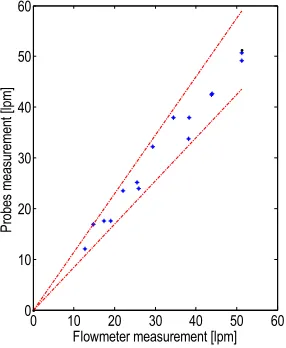
Validation of velocity profiles obtained with LDA and void fraction obtained from four-sensor conductivity
probes at same experiment conditions through
comparison of superficial liquid velocity measured with water flow meter. Errors inside ±10% limits have been obtained.
6. Conclusions
A methodology to measure the main magnitudes that characterize the two-phase flow is presented in this paper. Local interfacial area concentration, void fraction, chord
0,0 0,2 0,4 0,6 0,8 1,0 1,2 1,4
0 5 10 15 20 25 30
Liq
uid
v
elo
cit
y [
m
/s
]
Radial Position [mm]
jl=1m/s jg=0.05 TC jl=1m/s jg=0.05 TH jl=1m/s jg=0 TC
0,0 500,0 1.000,0 1.500,0 2.000,0 2.500,0 3.000,0 3.500,0 4.000,0 4.500,0
0,0 2,0 4,0 6,0 8,0 10,0 12,0 14,0
R
e [
-]
We [-]Fig 21. Map of Reynolds and Weber numbers. Liquid velocities are ranged from 0.5 to 3m/s whereas gas concentration were 4% to 36%. The different symbols show measurements obtained for different axial location, and the different colour show measurements obtained at different temperature. The legend is as follows: for all jl and jg ranges, ( ) L/D=22.4 and
TC, ( ) L/D=61 and TC, ( ) L/D=98.7 and TC, ( TA LOW) L/D=22.4 and TA, ( ) L/D=61 and TA, ( TA TOP) L/D=98.7 and TA,
( TH LOW) L/D=22.4 and TH, ( ) L/D=61 and TH, ( ) L/D=98.7 and TH, ( TRANSITION) transition or core peak distribution.
length, interfacial velocity and bubble size distribution for air-water flow through a vertical pipe are experimentally studied in order to provide an experimental database where temperature changes and transition effect have been taken into account. Experimental data from four-sensor conductivity probes and LDA system at different temperatures are presented in this paper to provide information about phase distribution inside the pipe, liquid and gas. The effects of temperature variation and turbulence over liquid phase velocity profile have been studied. Finally, experimental data has been evaluated to identify the transition from wall to core peak, using dimensionless Weber and Reynolds numbers.
Fig 22. Example of error check out using air flow meter, case
jl=1 m/s, jg=0.05-0.3 m/s and TC.
Acknowledgements
The authors sincerely thank the Spanish Science and Innovation Ministry for funding the project belonging to the Plan Nacional I+D, ENE2010-21368-C02-02 and ENE2010-21368-C02-01.
References
1. J.M. Delhaye, P.Bricard, J. Nucl. Engng. Des. 151,
pp. 65–77 (1994)
2. I. Kataoka, M. Ishii, A. Serizawa, Int. J. Multiphase
Flow, 12-4, pp.505-529 (1986)
3. T. Hibiki, M. Ishii, Int. J. Heat Mass Transfer, 42,
pp.3019-3035 (1999)
4. Q. Wu, M. Ishii, Int. J. Multiphase Flow, 25, 1,
pp.155-173 (1999)
5. T. Hibiki, M. Ishii, Z. Xiao, Int. J. Heat Mass
Transfer, 44, pp.1869-1888 (2001)
6. S. T. Revankar, M. Ishii, Int. J. Heat Mass Transfer,
36-12, pp.2997-3007 (1993)
7. S. Kim, X. Fu Y., X. Wang, M. Ishii, Int. J. Heat and
Mass Transfer, 43, 4101-4118 (2000)
8. T. Hibiki, M. Ishii, Z. Xiao, Int. J. Heat Mass
Transfer, 44, pp.1869-1888 (2001)
9. T. Hibiki, T. Hazuku, T. Takamasa, M. Ishii, AIAA
Journal, 47, 5, pp. 1123-1131 (2009)
10. Y. Taitel, D. Bornea, E. A. Dukler, AIChE J., 26,
345-354 (1980)
11. A. Serizawa, I. Kataoka, Phase distribution in
two-phase flow, Transient Phenomena in Multiphase
Flow, (Hemisphere, Washington DC, pp.179-224,
1988)
12. I. Zun, Transition from wall void peaking to core
void peaking in turbulent bubbly flow, Transient Phenomena in Multiphase flow (Hemisphere, Whashington DC, pp.225-245, 1988)
13. S. Mendez-Diaz, R. Zenit, S. Chiva, J. L.
Muñoz-Cobo, S. Martinez-Martinez, Int. J. Multiphase Flow,
43, pp. 56-61 (2012)
14. M. Ishii, Thermo-fluid Dynamic Theory of
Two-phase Flow (Eyrolles, Paris, 1975)
15. X. Shen, Y. Saito, K. Mishima, H. Nakamura, Int. J.
Multiphase Flow, 31, pp. 593–617 (2005)
16. M. Ishii, T. Hibiki, Thermo-fluid Dynamics of
Two-Phase Flow, Springer (2007)
17. W.K. Harteveld, R.F. Mudde, H. Van den Akker,
CJChE, 81, pp. 389–394 (2003)
18. M.J. Tummers, Investigation of a turbulent wake in
an adverse pressure gradient using laser Doppler anemometry (Ph.D. Thesis, Delft University of Technology, The Netherlands, 1999)
19. S. Turns, Introduction to Combustion (McGraw-Hill
Publishing Co, 2000)
20. D. C. Wilcox, Turbulence Modeling for CFD (DWC
Industries, 2006)
0 10 20 30 40 50 60 0
10 20 30 40 50 60
Flowmeter measurement [lpm]
P
ro
be
s
m
ea
su
re
m
en
t [
lp
m