(will be inserted by the editor)
DICE: Exploiting
All
Bivariate Dependencies in Binary and Multary
Search Spaces
Fergal Lane · R. Muhammad Atif Azad · Conor Ryan
the date of receipt and acceptance should be inserted later
Abstract Although some of the earliestEstimation of Dis-tribution Algorithms(EDAs) utilized bivariate marginal dis-tribution models, up to now, all discrete bivariate EDAs had one serious limitation: they were constrained to exploiting only a limitedO(d)subset out of all possibleO(d2) bivari-ate dependencies.
As a first we present a family of discrete bivariate EDAs that can learn and exploitall O(d2)dependencies between
variables, and yet have the same run-time complexity as their more limited counterparts. This family of algorithms, which we label DICE (DIscrete Correlated Estimation of distribution algorithms), is rigorously based on sound sta-tistical principles, and particularly on a modelling technique from statistical physics:dichotomised multivariate Gaussian distributions.
Initially [19], DICE was trialled on a suite of combi-natorial optimization problems over binary search spaces. Our proposeddichotomised Gaussian(DG) model in DICE significantly outperformed existing discrete bivariate EDAs; crucially, the performance gap increasingly widened as di-mensionality of the problems increased.
In this comprehensive treatment, wegeneraliseDICE by successfully extending it to multary search spaces that also allow forcategorical variables. Because correlation is not wholly meaningful for categorical variables, interactions be-tween such variables cannot be fully modelled by correlation-based approaches such as in the original formulation of DICE. Therefore, here we extend our original DG model to deal with such situations.
F. Lane·C. Ryan
CSIS Department, University of Limerick, Ireland E-mail: {Fergal.Lane, Conor.Ryan}@ul.ie
R. M. Atif Azad
School of Computing and Digital Technology, Birmingham City Uni-versity, UK
E-mail: [email protected]
We test DICE on a challenging test suite of combina-torial optimization problems, which are defined mostly on multary search spaces. While the two versions of DICE out-perform each other on different problem instances, they both outperform all the state-of-the-art bivariate EDAs on almost all of the problem instances. This further illustrates that these innovative DICE methods constitute a significant step change in the domain of discrete bivariate EDAs.
Keywords Dichotomised Gaussian models· Bivariate Estimation of Distribution Algorithms·Combinatorial Optimization
1 Introduction
Estimation of Distribution Algorithms (EDAs), often also called Probabilistic Model Building Genetic Algorithms (PMBGAs), are an important optimization paradigm within Evolutionary Computation. They are stochastic optimization methods that guide the search for a global optimum by build-ing and samplbuild-ing explicit probabilistic models. Traditional search operators like mutation and crossover are instead re-placed by a probabilistic model.
Many EDA variants have been developed for both con-tinuous and discrete problem domains. Some of the earliest EDAs used relatively simple univariate models, for example, the Univariate Marginal Distribution Algorithm (UMDA) [25], Population-Based Incremental Learning(PBIL) [1] and theCompact Genetic Algorithm(cGA) [14]. Such uncom-plicated models were, obviously, unlikely to suffice to tackle more difficult and intractable problems. There has been a long and natural progression towards the use of more com-plex models able to capture complicated problem dependen-cies and structures.
the development of this field. Such bivariate models are po-tentially much more expressive than univariate models. For discrete spaces, a well known example of a bivariate EDA would beMutual Information Maximizing Input Clustering (MIMIC) [7].
However, successively more expressive models have been investigated. Perhaps the most popular general EDA mod-elling approach has been graphical models and Bayesian networks. Some discrete search space examples would be the Bayesian Optimization Algorithm (BOA) [27] and the Estimation of Bayesian Networks Algorithm (EBNA) [9], and, in continuous search spaces, the Estimation of Gaus-sian Network Algorithm (EGNA) [20]. However, increas-ing expressiveness has almost invariably gone hand in hand with added computational costs and configurational com-plexities.
In this paper, we explore a novel bivariate EDA approach for discrete search spaces, based on dichotomised multivari-ate Gaussian distributions, that is no longer hindered by this constraint. These models have the attractive property of cap-turing and exploiting allO(d2)bivariate interactions between thedvariables of a problem domain. As far as these authors are aware, all bivariate marginal distribution models previ-ously used in discrete space EDAs were restricted to using justO(d)of these bivariate interactions.
The structure of the paper is as follows. Section 2 de-scribes previously developed bivariate EDAs. The dichotom-ised Gaussian(DG) model that DICE utilizes has its origins in the literature on the simulation of correlated multivariate Bernoulli variables. Section 3 begins with a brief survey of this literature. The bulk of this section, however, is devoted to a detailed description of the DG model and its implemen-tation. Section 4 describes an extended version of the basic DG model developed to cope with categorical variables in multary search spaces. Section 5 details our suite of com-binatorial optimization problem domains, the bivariate EDA algorithms we compare them with, and other experimental details. Section 6 presents results and analysis for these ex-periments. Finally, in section 7, we give our conclusions and lay out some ideas for future work.
2 Bivariate EDAs
2.1 Continuous Bivariate EDAs
In continuous spaces, models capable of efficiently captur-ing all bivariate marginal distributions are readily available and easy to use, e.g. the family of multivariate Gaussian distributions. EDAs like EMNA and theCovariance Matrix Adaptation Evolution Strategy(CMA-ES)1[13] , which uti-1 Strictly speaking, CMA-ES does not quite fall into the canonical
EDA framework. However, it shares almost all of the core features of a typical EDA.
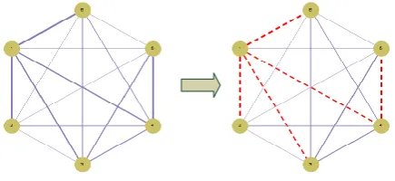
Fig. 1: The relative thicknesses of edges in the first graph represent rel-ative interaction strengths between six search space variables. Dashed red edges in the second graph represent the resulting constructed MST. Only edges/dependencies in the tree are exploited in these approaches.
lize such models have, therefore, long been widely available and used. TheEstimation of Gaussian Network Algorithm (EGNA)[20] is another continuous EDA that, at least in part, uses Gaussian distribution techniques. When there has been a need for even more expressive continuous models, several past authors have utilizedGaussian Mixture Models(GMMs) based on weighted mixtures of several multivariate Gaussian distributions [22].
2.2 Discrete Bivariate EDAs
For discrete spaces, the only bivariate EDAs available up-to-now have used restricted bivariate interaction models. MIMIC, mentioned earlier, greedily constructs a sequential chain of the most significantO(d)individual bivariate marginal dis-tributions. Building such chains or trees is the principal mod-elling strategy in existing discrete bivariate EDAs. Combin-ing Optimizers with Mutual Information Trees(COMIT) [2], and theBivariate Marginal Distribution Algorithm(BMDA) [28] are other examples. COMIT was essentially an exten-sion of MIMIC. Whereas, ford-dimensional problems with d dependent variables, MIMIC greedily constructed a se-quential chain ofO(d)individual bivariate marginal distri-butions, COMIT used a more generalO(d)dependency tree structure. MIMIC, COMIT and BMDA are all based on chains or trees ofd−1 individual bivariate marginal distributions.
at most one parent). However, even if this approach identi-fies and makes use of theO(d)out ofO(d2)most significant pairwise interactions, it still is the case that the vast majority are discarded. This may increasingly impact on model accu-racy as problem dimensionality increases. The BMDA algo-rithm also uses essentially the same procedure. The princi-pal difference is that it uses Pearson’s chi-squared estimator instead of mutual information to score bivariate variable in-teractions.
In [31], an interesting variation on such tree-based algo-rithms is given. Their algorithm, EDA based on Mixtures (EDAM), simply uses random trees (avoiding this costly O(d2)step). A mixture of ten such random trees was used as their EDA model in experiments. In essence, this algo-rithm reduces computational cost at the expense of some model accuracy. Despite randomly constructing the depen-dency trees, they claim their algorithm, nonetheless, per-formed similarly to MIMIC on tests.
A small number of authors have previously used mul-tivariate Gaussian copula models in EDAs. An example of this, which has some relevance to our work is [16]. There are some similarities between our approach and the algo-rithm given in section III of that paper. Their algoalgo-rithm is potentially capable of learning and exploiting all the bivari-ate marginal dependencies in the continuous problem do-mains examined in their paper. However, their method is not practical as a technique for discrete search spaces.
2.3 Computational Cost
A seeming advantage of previous MST techniques is the rel-atively lowO(d2)cost in building such a model (the main cost is the construction of the MST). However, even if these models identify and use only theO(d)most significant inter-actions, allO(d2)bivariate interaction strengths for a pop-ulation of size n must still be estimated and scored (with computational costO(d2n)). This is the primary computa-tional bottleneck for MIMIC and other past discrete bivari-ate EDAs.
The cost complexity of our newdichotomised Gaussian (DG) bivariate EDA model, which will be described in de-tail later, isO(max(d,n)d2)per generation. However, gen-erally, to have a reasonable chance of accurately estimating allO(d2)bivariate interaction parameters, it is expected that the population size n should at least be d. Therefore, the computational cost of the DG model normally is still of the same order as this unavoidableO(d2n)bivariate EDA gener-ational cost; hence, computgener-ationally DICE isnotmore com-plex than past discrete bivariate EDAs despite exhaustively exploiting all the bivariate dependencies. This is a signifi-cant result.
3 The Dichotomised Gaussian Model
3.1 Simulation of Correlated Multivariate Bernoulli Variables
The literature concerning simulation (random generation) of correlated binary vectors has a decades long history. A multivariate Bernoulli variable (essentially a randomly gen-erated bit string) is, in principle, fully specified by 2d−1 parameters (in effect, the individual probabilities for every possible bit string of lengthdit can generate). There is usu-ally little practical hope of accurately learning so many pa-rameters from data. A more realistic goal is to learn the uni-variate marginal distributions of the variables and the more limited number ofO(d2)correlations between those vari-ables. Then, one constructs a multivariate Bernoulli variable with those same univariate distribution and correlation char-acteristics.
Usually, the ideal choice would be to use the maximum entropy distribution for which the means and correlations for the set ofd binary variables are constrained to the de-sired target values. In this case, the maximum entropy dis-tribution is actually the well-known Ising model. Unfortu-nately, it is not at all straightforward or cheap to find the particular Ising model that fits a desired set of mean and correlation constraints. It is also difficult and expensive (in-deed NP-complete beyond a certain temperature) to sample binary vectors from such a model. Therefore, many other more practical methods have been proposed for simulating such correlated binary vectors.
Examples would include [4] that proposed a method us-ing look-up tables of sizeO(d3), [21] that introduced two methods – one based on setting up a linear programming problem and another based on Archimedean Copulas, [11] that introduced an “iterative proportional fitting algorithm”, and [17] that represents a more recent copula approach to this problem.
3.2 The Dichotomised Gaussian Model
can also easily be extended to the more general case of gen-erating multary vectors with any given correlation structure and associated set of univariate marginal distributions.
3.2.1 Randomly Generating Multary Strings
The DG method randomly generates multary search space stringsω ∈Ω where each gene position can choose from two or more possible allele values. HereΩis ad -dimension-al multary search spaceΩ=∏di=1ZaiwhereZai={0, . . . ,ai−1}, so that each ai≥2 specifies thearityof the ith dependent
variable (gene) ωi. So, using this notation, the ith geneωi
(out ofdpossible genes) can take on one out of ofai
possi-ble allele values (ranging from 0 up toai−1). At the heart of
the DG model is ad-dimensional multivariate normal distri-butionN (0,Σ)and an associated set of thresholds:
T =ntkb|k∈ {1, . . . ,d},b∈ {0, . . . ,(ak−2)}
o
The multivariate normal distribution is used to randomly generate ad-dimensional continuous vectorx∈ℜd. Each individual variablexiwill have a univariate marginal
distri-bution in ℜ with the usual Gaussian bell-shaped distribu-tion (with a mean of 0 and a variance of 1). The thresh-old values inT are used to convert thisd-dimensional ran-domly generated continuous vectorxinto ad-dimensional discrete multary stringω. Each variableωi, with arityai ,
will haveai−1 increasing threshold values associated with
it:t0
i <ti1· · ·<t ai−2
i which partitionℜintoaidisjoint
inter-vals:
Ki0= −∞,ti0,Ki1= ti0,ti1, . . . ,Kai−1
i =
tai−2
i ,∞
So, for example, ifxihappens to fall in the particular interval
Kc
i, then we setωi=c.
The basic operation of this method is, therefore, straight-forward: we first generate multivariate normal vectors ac-cording toN (0,Σ)and then dichotomise these using the set of thresholdsT to produce random multary strings.
3.2.2 Configuring the DG Model
The goal of the DG method is to allow the random gener-ation of multary search space vectorsω ∈Ω so that these conform to a set of desired univariate marginal density func-tions{pω
i (c)}i, wherep ω
i (c) =Pr{ωi=c}, and according to
a target set of variable (gene) correlationsri jgiven in ad×d
gene correlation matrix(R)i,j=ri j. Usually, the{pωi (c)}i
are empirical univariate marginal densities estimated from normalized allele frequency counts in the population, andR is a sample correlation matrix estimated from a population of selected search space points. Once we have our target es-timates forRand{pω
i (c)}i, then three further steps need to
be followed to properly configure the DG model (see Algo-rithm 1):
Algorithm 1Steps to configure the DG model
1: Calculate the set of threshold valuesT. These are chosen to repli-cate the target univariate marginal densitiespω
i(c). CalculatingT
has computational complexityO(a)wherea=Σid=1aiand empiri-cally estimating the{pω
i(c)}ifrom the population has costO(d n).
2: Calculate the correlation matrixΣ. The multivariate normald×
dcorrelation matrix(Σ)i,j=ρi jis constructed to ensure that the
correlations corr(ωi,ωj)in the generated multary stringsωmatch the target gene correlation matrixR. CalculatingΣhas costO(a2) and empirically estimatingRhas costO(d2n).
3: If necessary, use a nearest correlation matrix algorithm to repair
Σ(to reconcile any conflicting gene correlation targets). This has costO(d3).
Fig. 2: Illustration of calculating thresholds for a geneωiwith four
possible allele values and specific occurrence probabilities for each of these alleles.
Allele Values 0 1 2 3 Univariate Marginal Densities piω(.) 0.25 0.15 0.4 0.2
Cumulative Densities Piω(.) 0.25 0.4 0.8 1
Threshold Values -0.675 -0.253 0.842 ∞
Threshold values
0.675
Interval for allele value 1: Ki1
Interval for allele value 0: Ki0
Interval for allele value 2: Ki2
Interval for allele value 3: Ki3
0.253 0.842
0.25 0.15 0.4 0.2
Probability of Gaussian being in interval for allele value 0:
piω(0)
Probability of Gaussian being in interval for
allele value 3: piω(3)
3.2.3 Calculating the Threshold Values
We set the thresholds to exactly replicate the target univari-ate marginal densities{pω
i (c)}i. LetP ω
i (c) =Pr{ωi≤c}be
the targetcumulative distribution function(CDF) for vari-ableωi, which we can calculate as Piω(c) =∑ck=0pωi (c).
If we were thresholding simple uniform U(0,1)distribution variables (rather than normal variates), then these CDF den-sity values could be directly used as the thresholds. How-ever, since we are dichotomising normal distribution vari-ables, then we must first use the standard inverse normal CDF functionΦ−1(x)to map these to suitable correspond-ing normal threshold values:
ti0=Φ−1(Pω
i (0)), . . . ,tik=Φ
−1(Pω
i (k)), . . .
It can be easily verified that the univariate marginal densities of the resulting randomly generated multary vectorsω will indeed equal{pω
3.2.4 Replicating Gene Correlations
In step 1, we have already replicated the univariate marginal densities of our target discrete distribution. If we went no further and simply used a vector ofd independent normal variates with diagonalΣ, in our multivariate normal distri-butionN (0,Σ), then, in effect, we would have constructed a univariate EDA like PBIL or UMDA. However,(Σ)i j=ρi j
hasO(d2)free parameters for us to tune. After empirically estimating the matrix(R)i,j=ri jof correlations between the
search space variables in the selected population, we then adjust eachρi jso that the resulting correlation corr(ωi,ωj)
between variablesiand jin the generated random multary vectorωequals the desired target valueri j.
We can deal with each pair of variablesωiandωj
sepa-rately in turn. Their thresholds inT have already been cal-culated. Unfortunately, we cannot simply setρi jequal tori j.
However, for any possible value of ρi j, we can efficiently
calculate what the resulting corr(ωi,ωj)would be.
Only cheap-to-compute functions from the standard math-ematical toolbox are needed. We use the standard bivariate normal CDF functionΨ2(x,y;ρ)to calculate bivariate
marg-inal CDFs for the generated vectorωas:
Pω
i j(b,c) =Prob
ωi≤b∩ωj≤c =Ψ2
tib,tcj;ρi j
,i6=j
For convenience, if we also definePω
i j(b,c)to be 0
when-ever b<0 orc<0, then the bivariate marginal densities pω
ij(b,c) =Prob
ωi=b∩ωj=c forω can be expressed
and easily calculated as: pω
ij(b,c) =Pi jω(b,c)−Pi jω(b−1,c)−
Pω
i j(b,c−1) +Pi jω(b−1,c−1)
From these density values, the gene correlations can be cal-culated as:
corr(ωi,ωj) = ai−1
∑
b=0aj−1
∑
c=0b c pω
i j(b,c)−E(ωi)E(ωj),
i6=j, where E(ωi) = ai−1
∑
b=0b pω i (b)
!
We numerically adjustρi j until the resulting calculated
gene correlation betweenωi andωj exactly equalsri j. As
pointed out in [24], this problem is monotonic and there is guaranteed to be a single unique solution forρi jlying within [−1,1]. Straightforward and efficient one-dimensional bi-section root-finding algorithms can be used to quickly solve for eachρi j. In our implementation, we used Brent’s
root-finding bisection method, which on average converged within only six iterations. Alternative descriptions of this approach can be found in [8] and [24]. This process is repeated to esti-mateρi jfor each pair of variables until eventuallyΣ is fully calculated.
3.2.5 Repairing the Correlation Matrix
If the resultingΣ is a valid correlation matrix, i.e. is pos-itive semi-definite, then configuration of the DG model is complete. Positive semi-definite means all eigenvalues are non-negativeλi≥0 in the eigenvector decomposition:Σ= QDQT whereD=diag(λi).Σ may not always be positive
semi-definite due to incompatibilities, under this method, between different gene correlation targets in R. However, efficientcorrelation matrix repairalgorithms exist that can then replaceΣwith its nearest valid correlation matrix, cal-culated in terms of the Frobenius matrix norm.
A paper by Nicholas Higham [15] introduced the first al-gorithm for finding, for any arbitrary real matrix, its nearest valid correlation matrix. This method was based on Djik-stra’s “alternating projections method” and had linear con-vergence. However, later Newton-method based algorithms have been developed with fast quadratic convergence [29]. We used a publicly available2C-code version of this Newton-based algorithm. Our implementation of DICE is available from:https://github.com/FergalLane/DICE.
A simpler method, though not examined here, which we have found empirically almost as effective, is covariance matrix repair. The nearest valid covariance matrix toΣ is given byΣ+=Qdiag(max(λi,0))QT.Σ+ can then easily be converted back into a correlation matrix by renormaliza-tion:Σi j=
Σi j+
q
Σii+Σ+j j .
Both of these repair approaches have costO(d3)(due to the matrix operations involved). As can be seen from Al-gorithm 1, configuring the DG model each generation has an overall computational cost ofO(max(a2,d2n,d3)). Us-ing the DG model, generatUs-ing each new individual point has costO(d2)and new population,O(d2n). Unless allele arities are large, the effective cost complexity of the DG approach per generation isO(max(d,n)d2).
4 Extending the DG Model 4.1 Categorical Variables
DICE uses a correlation-based modelling approach. How-ever, variable correlations may not always be an entirely rel-evant measure for some types of multary search space. For example, in the graph colouring problem, which we will en-counter later, while numeric values can indeed be assigned to colours in a representation, a colouraveragein this case is not really meaningful. Colour is not a quantitative value for this problem; there is no inherent ordering between the possible colours. A variable holding such a qualitative value
2 Downloadable from:
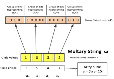
Fig. 3: An illustration of how a multary string is mapped to a binary representation
1 0 3 2
Multary String ω Allele values
Allele arities 3 5 4 3 a0 a1 a2 a3
Arity sum: a = ∑a i= 15 0 1 0 1 0 0 0 0 0 0 0 1 0 1 0
Binary String Representation Of a Multary String ω
Group of bits Representing
ω0=1
Group of bits Representing
ω1=0
Group of bits Representing
ω2=3
Group of bits Representing
ω3=2
Multary String Length= 4 Binary String Length=15
is usually termed a categorical or nominal variable. Cor-relation between the assigned colour values can still have a degree of usefulness. However, the inadequate treatment of categorical multary variables is a potential weakness in our original DICE approach. Therefore, in this section, we extend the original DG model to deal with this categorical case.
4.2 Binary Representations for Multary Strings
This extended model uses a binary representation for mul-tary strings. Suppose we have a multary string
ω ={ω0,ω1, . . . ,ωd−1} with individual variables ωi
hav-ing aritiesai. In our new approach, this multary string will
be represented as a longer bit stringbwhose total length is a=∑dk=1ak(thearity sum). Each multary variableωkis
rep-resented by a contiguous group ofakbits inb. Within this group, one and only one bit is allowed to be set. The posi-tion of this set bit corresponds to the allele value inωk. The
first bit being set corresponds to an allele value of 0, the sec-ond being set correspsec-onds to a value of 1 etc. Fig. 3 gives a concrete example of this mapping process.
In this representation, every possible allele value is al-located an individual bit position and is treated separately; correlations are calculated between individual allele values (collective averages and correlations between entire vari-ables are no longer calculated).
4.3 Generating Multary Strings With Categorical Variables
For a population of multary search space points expressed using thisa-dimensional bit string representation, a DG model can be built in the standard previously-described way (re-quiring the construction of ana×acorrelation matrix anda threshold values forT). This can then be used to generate
random bit strings with statistical characteristics matching the population. For example, the probability of any partic-ular bitk, which represents allele valuecat variableωi in
the population, being set will equal the univariate marginal densitypω
i (c)for that allele value.
However, a complication arises if we want to use this standard DICE approach to then randomly generate new in-dividuals. Within any group ofaibits representing a multary
variableωi, on average one of those bits will be set.
How-ever, sometimes more than one bit in the group will be set; at other times none at all will be set. To randomly simu-late multary strings, we need to be able to generate random binary vectors with the above statistical characteristics, but also constrained in such a way that always precisely one bit is set within each variable group (not just on average).
4.4 A Related Statistical Sampling Problem
Luckily, related problems have been studied in the field of stratified sampling in statistics [30]. Borrowing a technique from this area, we can indeed generate such bit strings with reasonable accuracy. This involves dichotomising the multi-variate normal vectorxgenerated by DICE in a new way.
The statistical topic, which closely relates to our needs, is the question of how best to randomly sample, without re-placement,nitems out of a population of sizeN, so that the selection probability for each itemkis proportional to some associated non-negative weightWk(we can also assume that
these weights have been normalized so that∑kWk=n).
Sev-eral techniques developed for doing this involve associat-ing with each itemkan independent random numberUk∼ U(0,1)and then using theWkas thresholds. If we select only items for whichWk≥Uk, i.e. for whichζk=WUk
k ≥1, then the resulting sample will have, on average,nitems exactly sampled proportional to their weightsWk. Unfortunately, the
resulting sample will only have a size ofnin expectation. Several authors have proposed techniques to remedy this issue. Ohlsson proposedSequential Poisson Sampling(SPS) [26], which simply selects thenitems with the largestζk
val-ues. He showed that this technique produces sampling prob-abilities close to the desired ones.
This example almost exactly mirrors our requirement to set/select exactly one (n=1) bit out of a group ofN=ai
bits that represent a multary variableωi. In DICE, each bitk
is set if its associated normal variablexkexceeds the
corre-sponding threshold valuetkinT. On average, exactly one bit per group is set. The principal difference with the statis-tical example is that we are using normal rather than uni-form random variates. However, using the standard normal CDF functionΦ(x), we can equivalently reformulate this in terms of the uniform distribution, puttingUk=Φ(xk)and
4.5 A New Thresholding Procedure
To always exactly set one bit in a group, we can use the SPS technique for thresholding: we first calculateζk=WUk
k for each bit in the variable group and only set the bit with the largestζkvalue. This alternative thresholding technique
will always produce a binary vector in a format that we can directly convert back into a multary string.
Rosen later created a similar sampling technique with even better properties: Pareto sampling [30]. In our work, we used his slightly different formula:ζk=Wk
(1−Uk)
Uk(1−Wk), setting only the single bit in each group with the largest such value. This new thresholding technique is easy to implement and is likely to produce univariate and bivariate marginal density properties close to the desired ones. The resulting overall DG model is also bigger and more detailed (learn-ing ana×arather than ad×d correlation matrix from the data). Exploiting more problem information could lead to improved performances. However, there are added costs (the cost per generation is nowO(max(a3,d2n))and, if there is not sufficient data to learn the bigger model, performance could potentially be negatively impacted.
5 Experimental Setup
Our overall goal was to test and compare the performance of DICE (using both original and extended dichotomised Gaus-sian models) with other existing discrete bivariate EDAs. Previously in [19], we only tested DICE on problem do-mains with binary search spaces. This time our test suite contains mostly problem domains with multary search spaces. To ensure an absolutely fair model comparison, we used the same basic EDA algorithm with identical settings with each EDA model.
5.1 EDA Algorithm Settings
All the EDAs used a population of 200 individuals. All al-gorithms were run for 100 generations. At each iteration, 200 new individuals were generated. We did this by going through all 200 existing individuals and, with probability pm, either mutating it (by picking one variable at random
and modifying its allele value) or, otherwise, replacing it en-tirely with an individual randomly generated using the cur-rent EDA model. Such a strategy was found to improve the performance of all EDAs we were testing. We used a setting ofpm=0.5 for all EDAs (empirically this particular setting
was determined to most boost general EDA performances). The 100 fittest individuals in the new population were then selected and used in updating the probability model. All the probabilistic EDA models were constructed, at each
iterationt, using a setHt∗of univariate and/or bivariate marg-inal densities (estimated from current and previous selected populations). We used an exponentially-decaying weighted average of previously encountered population density his-tograms. A model decay parameterτ ∈[0,1] was used to determine the factor at which the previous model was dis-counted at each iteration. So the new EDA modelHt∗would be the weighted combination:Ht∗= (1−τ)Ht+τHt∗−1of
the just previously discounted modelHt∗−1and the most re-cent selected population histogramHt. Extensive empirical
testing determined thatτ=0.75 was the best general setting for the EDAs on the problem test suite we examined here. An identicalτ=0.75 setting was used for all runs. Batches of 100 runs were used to produce all the experimental re-sults given below (except for MAX-SAT and graph colour-ing where 200 runs were used). We tested the EDAs on a range of dimensionalities:d=10,20, . . . ,100 for all prob-lem domains.
We compared our original DICE EDA, and the new ex-tended version,CategoricalVariable-DICE (CV-DICE), against a simpleUnivariate EDA(UEDA) model and the three prin-cipal discrete bivariate EDA models available in the liter-ature. These were the MST-based BMDA model (using the Pearson chi-squared statistic), the MST-based MIMIC model (scoring interactions using mutual information) and an inex-pensive random tree (EDAM) model where a mixture of ten randomly chosen dependency tree structures was used (the same model used in [31]).
5.2 Problem Test Suite
Several well-known combinatorial optimization problem do-mains, all defined on either binary or multary search spaces, were used; these are described in more detail in Table 1. All of these problem domains generated new fitness functions for every run by randomly sampling a new set of weights. We deliberately chose such problem domains because they readily scale to higher dimensions, and we wanted to test the performance of these models on search spaces of varying di-mensionalities.
Some, but not all, of the problem domains previously used in [19] had straightforward natural extensions to mul-tary search spaces. Mulmul-tary search spaces in this study used an arity of 4 for all variables (except for graph colouring, which used 3 colours and an arity-3 representation). Mul-tary versions of QUBO and CUBO (Cubic Unconstrained Binary Optimization) were used that simply replaced binary variables with integer ones (and the formulas rescaled ap-propriately).
from [6]:c=4.258d+58.26d13 to place it at the phase tran-sition point for SAT (similarly for 3-graph colouring).
In [23], some non-binary search space versions of NK Landscapes were developed. One of these,Nominal NK Land-scapes, was a simple multary extension of the original where the fitness component functionsFiwere also allowed to
ac-cept multary allele values. This NK Landscape variant has a categorical variable structure. We wished to also include a multary version of NK Landscapes that had variables with non-categorical (ordinal or quantitative) properties. There-fore, we constructed a novel but simple multary NK Land-scape based on tessellations (or random cuts). Associated with each variableikin everyFifunction (see Table 1) is a
randomly generated cut valueci∼U(0,ai−1). Allele
val-ues below this cut are treated by theFifunctions as 0, while
allele values greater than this cut point are treated as 1 (en-suring that allele values further apart are more likely to be “cut” and assigned different random values).
We also included the Quadratic Knapsack Problem, which has a significant associated literature. We use the classic form of the problem as originated by Gallo [10].
6 Results and Analysis
Fig. 4 details the EDA performances on both types of NK Landscapes. Like other graphs in this section, mean best run fitness for the EDA models for individual problem domains is plotted. Clearly, DICE (using the original DG model) and CV-DICE (using the new extended model) are the best per-formers in all cases. CV-DICE has better performance in more cases. However, for higher dimensions on the Nom-inal NK Landscapes with K=3,4, DICE has better perfor-mances. The reasons for this will need further investigation; it is possible our populations contain an insufficient number of individuals for the more detailed CV-DICE model to be fully learned, particularly at higher dimensions.
Fig. 5 gives EDA performances on the Multary QUBO and CUBO problem domains. DICE and CV-DICE have the overall best performances on QUBO. DICE spectacularly outperforms all other EDAs on multary QUBO. CV-DICE is still clearly the runner-up, but lags far behind DICE. This is perhaps unsurprising given that the variable structure is very much quantitative, rather than categorical, for this problem domain.The performance gaps between DICE and CV-DICE and back to the others are all significant at least a 99% level of significance using the two-tailed Student’s t-test (for all further comparisons a 99% level of significance using this test can be assumed unless specified otherwise).
For nine out of the eleven problem domains in this test suite, DICE and CV-DICE have the best performances. Mul-tary CUBO is one of two cases where this did not hold. In [19], DICE could successfully cope with moderate numbers
of higher order interactions. Here, perhaps the much denser O(d3) number of order-three variable interactions simply overwhelms theO(d2)-parameter DG model.
For the two problem domains, 3-Uniform MAX-SAT and 3-Graph Colouring, that made use of phase transition theory, the performance margins between all EDAs were nu-merically very small and graphically hard to see. The op-timizers quickly were able to satisfy almost all colour or clause constraints. However, at the phase transition point, while there may be many local optima coming relatively close to satisfying all clauses/colour constraints, there will be very few or no points satisfying all of them. The real dif-ficulty with such problem domains is in finding solutions which satisfy the final small number of remaining constraints.
For these two problem domains, we ran batches of 200 rather than 100 simulations in order to better statistically dif-ferentiate between such small performance gaps. To further simplify comparison of results and reduce standard errors, we give combined mean best run fitnesses, averaged across all dimensionalities, for these problem domains. These com-bined results are given in table form in Table 2 rather than as graphs. Similar performance figures for the Quadratic Knap-sack problem domain are also given (performance gaps were also small in this case).
CV-DICE performs best on the Quadratic Knapsack and DICE is in second place. DICE and CV-DICE perform best on MAX-SAT with their performance gap not being statis-tically significant; there should not really be a significant performance gap as both DG models should perform almost identically on binary search spaces. The performance gap back to BMDA and MIMIC is also not quite statistically sig-nificant.
For 3-Graph Colouring, MIMIC and BMDA beat CV-DICE and CV-DICE into third and fourth places. However, at the 3-Graph Colouring phase transition, each vertex is con-nected on average with only 4.687 other vertices. For such sparse limited-dependency graphs, simpler tree-based mod-els may be adequate (the added expressivness of the DG model may confer no real advantage in this case).
Overall, for nine out of eleven problem domains, both DICE and CV-DICE have superior performances to all other EDAs.
7 Conclusions
In this paper, we generalise the first fully bivariate model for discrete EDAs to cover both binary and multary search spaces. A key innovation was a treatment of categorical vari-ables which are not directly amenable to correlational mod-els. A key feature of the DICE family is its computational complexity: in its original form, despite exploiting allO(d2)
Table 1: Problem Domain Test Suite Details
Problem Domain Category Ref Fitness Function Formula/Details
Multary QUBO Multary [3] f(ω) =∑di,j=1wi j(2si−1)(2sj−1),wi j∼N(0,d12),si=
ωi
ai−1
Multary CUBO Multary [12] f(ω) =∑di,j,k=1wi jk(si)(sj)(sk),wi j∼N(0,d13),si=
ωi
ai−1
Nominal NK-Landscapes
Categorical Multary
[23]
K=2,3,4;f(ω) =√1 d∑
d
i=1Fi(ωi;ωi1, . . . ,ωiK)where theijare chosen randomly without
replacement; eachFireturns a unique random normally distributed value for every unique K+1-allele combination encountered.
Tessellation NK-Landscapes
Multary
Same as above except a randomcut value cik∼U(0,aik−1)is associated with each variable in everyFiand f(ω) =√1
d∑ d
i=1Fi(Iωi≥ci; Iωi1≥cik, . . . ,IωiK≥ciK)so allele values on the same side of
a cut are treated identically, and those on opposites sides, differently. 3-Uniform
MAX-SAT
Binary [6] The number of clausescis set using the phase transition formula in [6].
3-Graph Colouring Categorical Multary
[18] Fitness is the number of edges in the graph whose vertex colours differ; the graph connectivity is set as close as possible to 4.687 to be at the phase transition.
Quadratic Knapsack Problem
Binary [10] f(ω) = 1
d∑ d
i,j=1pi jωiωjsubject to∑dj=1wjωj≤c, eachpi jis non-zero with probability Λ=0.33,pi j∼U(1,50),wi∼U(1,100)andc∼U[50,∑dj=1wi],ωi∈ {0,1}
Fig. 4: Mean Best Run Fitnesses for the EDA models on the Nominal NK and Tessellation NK Landscapes
● ● ● ● ● ● ● ● ● ● ■ ■ ■ ■ ■ ■ ■ ■ ■ ■ ◆ ◆ ◆ ◆ ◆ ◆ ◆ ◆ ◆ ◆ ▲ ▲ ▲ ▲ ▲ ▲ ▲ ▲ ▲ ▲ ▼ ▼ ▼ ▼ ▼ ▼ ▼ ▼ ▼ ▼ ○ ○ ○ ○ ○ ○ ○ ○ ○ ○
0 20 40 60 80 100 5 6 7 8 Dimension d Mean Best Run Fitness
Nominal NK Landscape, K=2
● ● ● ● ● ● ● ● ● ● ■ ■ ■ ■ ■ ■ ■ ■ ■ ■ ◆ ◆ ◆ ◆ ◆ ◆ ◆ ◆ ◆ ◆ ▲ ▲ ▲ ▲ ▲ ▲ ▲ ▲ ▲ ▲ ▼ ▼ ▼ ▼ ▼ ▼ ▼ ▼ ▼ ▼ ○ ○ ○ ○ ○ ○ ○ ○ ○ ○
0 20 40 60 80 100 4.5 5.0 5.5 6.0 Dimension d Mean Best Run Fitness
Nominal NK Landscape, K=3
● ● ● ● ● ● ● ● ● ● ■ ■ ■ ■ ■ ■ ■ ■ ■ ■ ◆ ◆ ◆ ◆ ◆ ◆ ◆ ◆ ◆ ◆ ▲ ▲ ▲ ▲ ▲ ▲ ▲ ▲ ▲ ▲ ▼ ▼ ▼ ▼ ▼ ▼ ▼ ▼ ▼ ▼ ○ ○ ○ ○ ○ ○ ○ ○ ○ ○
0 20 40 60 80 100 4.0 4.2 4.4 4.6 4.8 Dimension d Mean Best Run Fitness
Nominal NK Landscape, K=4
● UEDA
■ EDAM
◆ BMDA
▲ MIMIC
▼ DICE
○ CV-DICE
● ● ● ● ● ● ● ● ● ● ■ ■ ■ ■ ■ ■ ■ ■ ■ ■ ◆ ◆ ◆ ◆ ◆ ◆ ◆ ◆ ◆ ◆ ▲ ▲ ▲ ▲ ▲ ▲ ▲ ▲ ▲ ▲ ▼ ▼ ▼ ▼ ▼ ▼ ▼ ▼ ▼ ▼ ○ ○ ○ ○ ○ ○ ○ ○ ○ ○
0 20 40 60 80 100 3 4 5 6 7 8 Dimension d Mean Best Run Fitness
Tessellation NK Landscape, K=2
● ● ● ● ● ● ● ● ● ● ■ ■ ■ ■ ■ ■ ■ ■ ■ ■ ◆ ◆ ◆ ◆ ◆ ◆ ◆ ◆ ◆ ◆ ▲ ▲ ▲ ▲ ▲ ▲ ▲ ▲ ▲ ▲ ▼ ▼ ▼ ▼ ▼ ▼ ▼ ▼ ▼ ▼ ○ ○ ○ ○ ○ ○ ○ ○ ○ ○
0 20 40 60 80 100 3 4 5 6 7 8 Dimension d Mean Best Run Fitness
Tessellation NK Landscape, K=3
● ● ● ● ● ● ● ● ● ● ■ ■ ■ ■ ■ ■ ■ ■ ■ ■ ◆ ◆ ◆ ◆ ◆ ◆ ◆ ◆ ◆ ◆ ▲ ▲ ▲ ▲ ▲ ▲ ▲ ▲ ▲ ▲ ▼ ▼ ▼ ▼ ▼ ▼ ▼ ▼ ▼ ▼ ○ ○ ○ ○ ○ ○ ○ ○ ○ ○
0 20 40 60 80 100 3 4 5 6 7 8 Dimension d Mean Best Run Fitness
Tessellation NK Landscape, K=4
● UEDA
■ EDAM
◆ BMDA
▲ MIMIC
▼ DICE
○ CV-DICE
Fig. 5: Mean Best Run Fitnesses for the EDA models on the Multary QUBO and CUBO problem domains
● ● ● ● ● ● ● ● ● ● ■ ■ ■ ■ ■ ■ ■ ■ ■ ■ ◆▲ ◆ ◆ ◆ ◆ ◆ ◆ ◆ ◆ ◆ ▲ ▲ ▲ ▲ ▲ ▲ ▲ ▲ ▲ ▼ ▼ ▼ ▼ ▼ ▼ ▼ ▼ ▼ ▼ ○ ○ ○ ○ ○ ○ ○ ○ ○ ○
0 20 40 60 80 100
0 1 2 3 4 5 6 Dimension d Mean Best Run Fitness Multary QUBO ● ● ● ● ● ● ● ● ● ● ■ ■ ■ ■ ■ ■ ■ ■ ■ ■ ◆ ◆ ◆ ◆ ◆ ◆ ◆ ◆ ◆ ◆ ▲ ▲ ▲ ▲ ▲ ▲ ▲ ▲ ▲ ▲ ▼ ▼ ▼ ▼ ▼ ▼ ▼ ▼ ▼ ▼ ○ ○ ○ ○ ○ ○ ○ ○ ○ ○
0 20 40 60 80 100
0.80 0.85 0.90 0.95 1.00 1.05 1.10 Dimension d Mean Best Run Fitness Multary CUBO ● UEDA ■ EDAM ◆ BMDA ▲ MIMIC ▼ DICE
Table 2: Combined Mean Best Run Fitnesses for the EDA models av-eraged across all Problem Sizes for the 3-Graph Colouring, 3-Uniform Knapsack and Quadratic Knapsack problems domains
Problem Domains EDA
Model
3-Uniform MAX-SAT
3-Graph Colouring
Quadratic Knapsack UEDA 236.04±0.03 53.09±0.02 230.10±0.03 EDAM 235.77±0.03 52.73±0.02 227.85±0.03 BMDA 236.18±0.03 53.61±0.02 228.28±0.03 MIMIC 236.18±0.03 53.69±0.02 228.27±0.03 DICE 236.24±0.03 53.34±0.02 230.38±0.03 CV-DICE 236.20±0.03 53.50±0.02 230.81±0.03
complex than its approximate counterparts that only explore O(d) dependencies. In a majority of cases in our experi-ments, the extended DICE outperformed the original DICE model. Overall, however, the two DICE versions outperformed all the other state-of-the-art discrete bivariate EDAs on nine out of eleven problems in the test suite.
7.1 Future Work
The DG model has the potential to adapt other algorithms from continuous domains, particularly those based on Gaus-sian distributions, to discrete spaces. CMA-ES [13], a popu-lar and powerful EDA-like optimizer for continuous search spaces, would be a promising candidate for such treatment.
The DG model would be a good candidate for knowl-edge incorporation. Correlation matrix repair can also be performed using various forms ofweightedFrobenius norms (rather than the standard norm we use in this paper). In-creased weights can be used to give inIn-creased priority and protection to variable interactions learned to be more signif-icant.
Acknowledgements This work was supported with the financial sup-port of the Science Foundation Ireland grant 13/RC/2094.
References
1. Baluja, S., Caruana, R.: Removing the genetics from the standard genetic algorithm. In: 12th Int. Conf. on Machine Learning. pp. 38–46 (1995)
2. Baluja, S., Davies, S.: Using optimal dependency-trees for com-binational optimization. In: 14th Int. Conf. on Machine Learning. pp. 30–38 (1997)
3. Boros, E., Hammer, P., Tavares, G.: Local Search Heuristics for Quadratic Unconstrained Binary Optimization (QUBO). Journal of Heuristics 13(2), 99–132 (Apr 2007)
4. Caprara, A., et al.: Generation of antipodal random vectors with prescribed non-stationary 2-nd order statistics. IEEE Transactions on Signal Processing 62(6), 1603–1612 (2014)
5. Chow, C., Liu, C.: Approximating discrete probability distribu-tions with dependence trees. IEEE Transacdistribu-tions on Information Theory 14(3), 462–467 (1968)
6. Crawford, J., Auton, L.: Experimental results on the crossover point in random 3-SAT. Artificial intelligence 81(1), 31–57 (1996) 7. De Bonet, J., Isbell, C., et al.: MIMIC: Finding optima by esti-mating probability densities. Advances in Neural Information Pro-cessing Systems pp. 424–430 (1997)
8. Emrich, L., Piedmonte, M.: A method for generating high-dimensional multivariate binary variates. The American Statisti-cian 45(4), 302–304 (1991)
9. Etxeberria, R., Larranaga, P.: Global optimization using Bayes-ian networks. In: Second Symposium on Artificial Intelligence (CIMAF-99). pp. 332–339. Habana, Cuba (1999)
10. Gallo, G., et al.: Quadratic knapsack problems. In: Combinatorial Optimization, pp. 132–149. Springer (1980)
11. Gange, S.: Generating multivariate categorical variates using the iterative proportional fitting algorithm. The American Statistician 49(2), 134–138 (1995)
12. Glover, F., Hao, J.K., Kochenberger, G.: Polynomial uncon-strained binary optimisation – part 2. International Journal of Metaheuristics 1(4), 317–354 (2011)
13. Hansen, N., Kern, S.: Evaluating the CMA evolution strategy on multimodal test functions. In: PPSN VIII. pp. 282–291 (2004) 14. Harik, G., Lobo, F., et al.: The Compact Genetic Algorithm. IEEE
Transactions On Evolutionary Computation 3(4), 287–297 (1999) 15. Higham, N.: Computing the nearest correlation matrix : a problem from finance. IMA Journal of Numerical Analysis 22(3), 329–343 (2002)
16. Hyrš, M., Schwarz, J.: Multivariate Gaussian copula in estimation of distribution algorithm with model migration. In: Foundations of Computational Intelligence (FOCI). pp. 114–119. IEEE (2014) 17. Jin, R., Wang, S., et al.: Generating spatial correlated binary data
through a copulas method. Science Research 3(4), 206–212 (2015) 18. Krz ˛akała, F.: How many colors to color a random graph? Cavity, complexity, stability and all that. Progress of Theoretical Physics Supplement 157, 357–360 (2005)
19. Lane, F., Azad, R., Ryan, C.: DICE: A new family of bivariate estimation of distribution algorithms based on dichotomised mul-tivariate Gaussian distributions. In: European Conference on the Applications of Evolutionary Computation. pp. 670–685. Springer (2017)
20. Larrañaga, P., Etxeberria, R., et al.: Combinatorial optimization by learning and simulation of Bayesian networks. In: 16th Conf. on Uncertainty in Artificial Intelligence. pp. 343–352 (2000) 21. Lee, A.: Generating random binary deviates having fixed marginal
distributions and specified degrees of association. The American Statistician 47(3), 209–215 (1993)
22. Li, B., Wang, X., Zhong, R., Zhuang, Z.: Continuous optimization based-on boosting Gaussian mixture model. In: 18th Int. Conf. on Pattern Recognition. vol. 1, pp. 1192–1195. IEEE (2006) 23. Li, R., Emmerich, M., et al.: Mixed-integer NK landscapes. In:
Parallel Problem Solving from Nature (PPSN IX). pp. 42–51 (2006)
24. Macke, J., Berens, P., et al.: Generating spike trains with speci-fied correlation coefficients. Neural Computation 21(2), 397–423 (2009)
25. Mühlenbein, H.: The equation for response to selection and its use for prediction. Evolutionary Computation 5(3), 303–346 (1997) 26. Ohlsson, E.: Sequential Poisson Sampling. Journal of Official
Statistics 14(2), 149 (1998)
27. Pelikan, M., Goldberg, D., Cantú-Paz, E.: BOA: The Bayesian op-timization algorithm. In: GECCO 1999. pp. 525–532 (1999) 28. Pelikan, M., Mühlenbein, H.: The bivariate marginal distribution
algorithm. In: Advances in Soft Computing, pp. 521–535 (1999) 29. Qi, H., Sun, D.: A quadratically convergent Newton method for
computing the nearest correlation matrix. SIAM journal on matrix analysis and applications 28(2), 360–385 (2006)