This paper was originally published by IWA Publishing. The author’s right to reuse
and post their work published by IWA Publishing is defined by IWA Publishing’s
copyright policy.
If the copyright has been transferred to IWA Publishing, the publisher recognizes the
retention of the right by the author(s) to photocopy or make single electronic copies
of the paper for their own personal use, including for their own classroom use, or the
personal use of colleagues, provided the copies are not offered for sale and are not
distributed in a systematic way outside of their employing institution.
Please note
that you are not permitted to post the IWA Publishing PDF version of your
paper on your own website or your institution’s website or repository.
If the paper has been published “Open Access”, the terms of its use and distribution
are defined by the Creative Commons licence selected by the author.
Full details can be found here: http://iwaponline.com/content/rights-permissions
Merged two-level optimization for optimal pump
operation of large scale urban water distribution system
Xi Jin and Wenyan Wu
ABSTRACT
Subsequent to the least cost design problem of water distribution systems (WDSs), optimal operation
is probably the most explored topic. Since 1970 a variety of methods have been developed to
address this problem. Although the proposed methods give theoretic ways for solving optimal
operation problems of WDSs, there are little successful application cases in practice, especially when
the methods were used to large scale WDSs due to too many decision variables. In consideration of
using fewer decision variables, the two-level optimal method is adopted in this paper. By abstracting
pump stations into high level reservoirs, the water distribution system hydraulic model can be
modified into a modality, which can be used infirst optimal level of two-level optimal method. Also,
by building on feasible pump combination database, a new optimal method in the second optimal
level will be proposed, and the proposed new method in the second optimal level will be embedded
into thefirst optimal level, so that the problem of results discordant in different levels will be solved.
By introducing new concepts and improving present optimal methods, a more practical optimal
operation method of water distribution system will be established. By applying in a large scale
practical water distribution system, the proposed method has been evaluated.
Xi Jin(corresponding author)
School of Civil Engineering and Architecture, Wuhan University of Technology Wuhan, Hubei,
China
E-mail:[email protected]
Wenyan Wu
Faculty of Arts and Creative Technologies, Staffordshire University,
Stafford, UK
Key words|decision support system, genetic algorithm, pump operation, water distribution system
INTRODUCTION
The operational cost of pumps in a water distribution system (WDS) represents a significant fraction of the total expendi-ture incurred in the operational management of WDSs worldwide. Pumps consume large amounts of electrical energy for pumping water from source to storage tanks and to demand nodes. Therefore, the goal of a pump scheduling problem is to minimize the total pump operational cost, while guaranteeing a competent network service. In most cases, this problem is equivalent to the minimization of pumping cost, while supplying water to consumers at ade-quate pressures (López-Ibáñez et al. ). In recent years, a significant amount of research has been focused on optimiz-ing pump operation schedules. Since 1970, a variety of conventional methods such as dynamic programming, linear programming (LP) and nonlinear programming were developed to address this problem. A review of some early
optimization approaches to pump scheduling can be found inOrmsbee & Lansey (). Price & Ostfeld () devel-oped an algorithm which enables iterative linearization of increasing or decreasing convex nonlinear equations and incorporating them into LP optimization models, which results in short solution times. However, the discrete (binary) nature of some variables and the size of the solution space are among the main difficulties of optimizing water dis-tribution systems operation (Van Dijk et al. ). Conventional optimization methods are not directly appli-cable for solving such problems, because these methods are suitable mostly for optimization problems which have only continuous variables, therefore population based methods such as evolutionary algorithms and various meta-heuristics were introduced to deal with the optimal pump scheduling problem. Mackle et al. () presented a single objective
optimization (electric energy cost) using genetic algorithms (GAs). Then,Savicet al. ()proposed a hybridization of a GA with a local search method, in order to optimize two objectives: electric energy cost and pumps maintenance cost. Fang et al. () solved optimization of the pump system with constant and variable speed pumps with multi-objective evolutionary algorithms (MOEAs) combined with a repair mechanism. As a result, evolutionary computation has proven to be a powerful tool to solve optimal pump-sche-duling problems (Benjamin et al. ). Although the methods mentioned above give theoretic methods for solving the optimal pump scheduling problem of WDSs, population based algorithms have the following drawbacks. First, they require a large number of the objective and constraint func-tion evaluafunc-tions which are not acceptable when these evaluations are expensive. Second, they are inefficient for sol-ving large scale problems. Third, these algorithms sometimes cannot locate a solution with high accuracy and as a result, they may produce only suboptimal solutions (Bagirov et al. ). In this situation, a two-level optimal concept was addressed on better effectiveness and efficiency of solving the optimal pump scheduling problem. In a methodology based on a two-level optimal concept, the optimal outflow and head of source nodes or elevated storage trajectory are determined in thefirst optimal level, and the optimal pump schedules will be determined in the second level, so that a complex optimal problem is divided into several relative sim-pler optimal problems.Ormsbeeet al.()proposed a two-level optimal methodology using elevated tank trajectory as the first level objective, and pump combinations as the second level objective. The optimal trajectory is determined using dynamic programming while the associated pump com-bination is determined using an explicit enumeration scheme. Kevin & Kofi ()developed a two-level optimal method-ology based on Ormsbee’s concept, and considered pump switches as a constraint of optimization model. Pump combi-nations were solved by dynamic programming. Due to the problem of the variables dimension, these methods are only applicable to small to mid-size systems with elevated storage. Zheng () developed a two-level optimal methodology regarding outflow and head of source nodes as the decision variables of thefirst level optimal problem. Thefirst level opti-mal problem is solved by the variable-metric method, and the pump combination result is obtained by the enumeration
scheme.Zhanget al.()presented a method using differ-ent algorithms to solve optimal pump combination problems for pump stations with or without variable speed pumps in the second level, so that the pump rotary speed can be regarded as decision variables and more rational and efficient pump combinations can be obtained.Yuanet al.() pro-posed a two-level methodology which determines outflow variables in the first level using the Wilson–Han–Powell method, and determines pump combination and pump rotary speed with a reduced gradient method. With the devel-opment of the two-level methodology, more effective and efficient optimal models addressed on large scale WDS opti-mal operation problems are presented. However, there are still some problems that hinder the optimization method to be applied in practice. In these problems, the most outstand-ing ones are as follows. (1) Since there is no determined pump schedules, only meta-models can be used in thefirst level optimization. However, the meta-model is not as robust as a hydraulic model, so the reliability of optimization result is low. (2) Another problem of the two-level optimiz-ation is discordant of results in different levels. Since the two levels are solved in totally different phases, the feasibility of thefirst level result cannot be examined by pump combi-nation information. So sometimes there is no feasible pump combination that can match the result of thefirst level.
For the purpose of solving these problems, a modified hydraulic model and pump combination database are intro-duced into the two-level method. By regarding pump stations as high level reservoirs, the hydraulic model of WDSs can be modified into a modality that can be used in thefirst opti-mal level of the two-level method, so that the defects of poor effect and low reliability of optimal results of thefirst optimal level solved with meta-models will be resolved. By building a database on feasible pump combination, a new optimal method in the second optimal level will be proposed. The sol-ving process of the second optimal level will be embedded into thefirst optimal level, so that the problem of discordant results in different levels will be solved.
OPTIMAL MODEL FORMULATIONS
the single objective optimization method, constraints will be added into the evaluation value by the weighting method or punish functions. Previous studies (Mackle et al. ; Bouloset al.) dealt with constraints by penalizing the objective function. This requires the definition of a penalty function and appropriate penalty values. Moreover, different penalty values are required for different types of constraints and the degree of violation of some of these constraints cannot be easily quantified. To avoid this, a multi-objective optimal model is built with three objectives: minimum elec-tricity cost, minimum amount of lower pressure service nodes and minimum error between two optimal levels. A multi-objective oriented solving method is used in the optimization.
Objectives
The pump energy cost depends on the energy price as well as on the amount of energy consumed. The minimum elec-tricity cost objective can be expressed by Equation (1):
Min:C¼X
S
i¼1
PiTt (1)
whereSis the set of source nodes,Piis the power consumed
by theith pump (kw),Tis the electricity tariff in the current period (¥/kwh), t is the length of the hydraulic time step (1 h).
The objective of minimum number of lower pressure ser-vice nodes is expressed by Equation (2):
Min:M¼X
N
i¼1
βi where: βi¼ 0 if
HiHmin 1 if Hi<Hmin
(2)
whereNis total demand nodes number,Hiis pressure ofith
node, andHminis the minimum service pressure required at
demand node.
The third objective value is the error between two opti-mal levels. During the second level optiopti-mal process, a candidate pump combination will be selected for each sol-ution according to the first optimal level result. In the pump combination database, discrete running conditions of all different pump combinations are recorded. Since
decision variables (outflow and head of source nodes) of first optimal level are continuous variables, it is hard to match thefirst optimal level result by a record from pump combination database exactly. So a neighbourhood region has to be generated by using the hydraulic results of each solution from thefirst level as central point and a designed length as the broader range. Records that fall into this neigh-bourhood region can be regarded as candidate pump combinations of this solution, and the flow difference between running conditions of the pump combination record and hydraulic result is the error between two optimal levels of this solution. This objective represents the ration-ality of the second optimal result. The less the error is, the more rational the second optimal result is. This error can be regarded as a measurement of difference between the modified hydraulic model simulation result and original hydraulic model simulation result. The error objective can be expressed by Equation (3):
Min:E¼X
S
i¼1
εi where
εi¼ ∞ if F
0
i∉(Fiθ,Fiþθ)
jFiFi0j if Fi0∈(Fiθ,Fiþθ)
(3)
whereFiis the outflow of theith source node of the
hydrau-lic result of solution,Fi’is the outflow of the candidate pump
combination. θ is the broader range that is set before the optimization process.∞is a very large number as a penalty for when no pump combination records fall into the neigh-bourhood region, it means that for the ith source node, there is no feasible pump combination that can match the first optimal level results.
Constraints
proposed method, the minimum pressure requirement is regarded as an objective value, so there are no constraints about demand nodes pressure criteria in the optimal model. In this study, EPANET is used as the hydraulic simu-lator for handling the constraints.
SOLVING METHODOLOGY
In the two-level optimal methods of previous studies, the first level and second level is totally divided as two parts. The second level will be run after the first level has been done. Since there are no detailed pump schedules in the first optimal level, so the cost objective value can only be calculated based on an average pump efficiency parameter assigned beforehand, and only a meta-model can be used to evaluatefitness of candidate solutions in thefirst optimal level. The introduction of an average pump efficiency par-ameter may lead to an error between cost objective values of thefirst optimal level and the second optimal level, and cannot guarantee the first level result is an optimal one. The meta-model can only be trained by historical data, so it cannot be used directly after WDS expansion or
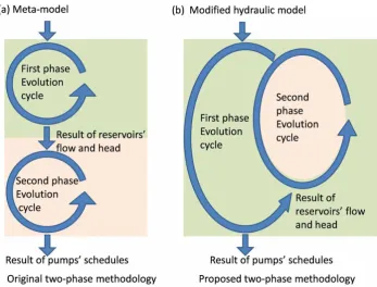
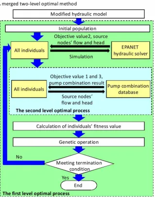
rehabilitation, and cannot be used to forecast WDS running condition in scenarios that have not happened, and cannot evaluate hydraulic constraints of the candidate scheme in detail, for example, the meta-model can only evaluate pressure constraints for certain nodes in WDS. These short-comings of the meta-model make the two-level optimal method not a robust methodology. To avoid these shortcom-ings, a merged two-level optimal method with a hydraulic simulator is proposed. In order to use a hydraulic simulator in thefirst level, a modification has to be carried out to the original WDS hydraulic model by transforming the pump stations into elevated reservoirs. In order to avoid the pro-blem of discordance between two levels’ results, the second optimal level process will be embedded into the first optimal level, and executed to each candidate solution in every evolved step. The difference between the proposed two-level optimal method and the previous two-level opti-mal method is shown inFigure 1.
Building pump combination database
The pump combination database will be used in the second optimal level. The records of running conditions of each
pump combination are stored in the database. For each source node, the pumps willfirst be organized into a set of pump combinations. Then the characteristic curves (Q-H, Q-E curves) of the parallel pump running conditions of each pump combination will be calculated by using charac-teristic curves of each pump of the combination. In the database, the characteristic curves for each pump combi-nation are recorded by discrete running condition sample points. In each running condition point, the parameters of flow, head, efficiency and power are recorded. The detailed process of building a pump combination database is described below. In general, it is rare to run all pumps in one pump station simultaneously, so a maximum amount of running pumps can be set for the pump station. With this limitation, the records in the pump combination dataset will be smaller, and the efficiency of the enumeration algor-ithm for the pump combination selection can be enhanced. The pumps and combinations of example pump station are shown inTable 1.
In the example pump station, there are three pump types A, B and C and the maximum number of running pumps is 4. The total combinations are listed in the ‘combination’ column. Each element in the‘combination’column is com-bined by pump type and its number (the number in brackets after the pump type), and there is no number and bracket if the number is 1.
For each pump combination, the running condition sample points of the Q-H characteristic curve will be calcu-lated by Q-H characteristic curves of pumps in combination, according to the rule of‘flow added in each head sample point’. The efficiency of each pump at running condition sample points can be obtained by the pump’s Q-E curve and itsflow parameter. The power of each pump at running condition sample points can be obtained byflow, head and
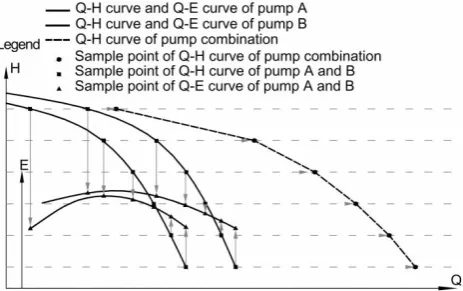
efficiency parameters. The total power is a summary of power of each pump in this pump combination. The total efficiency is the ratio of effective power and total power. The calculation concept of Q-H sample points of pump com-bination and efficiency sample points of each pump is illustrated by an example of pump combination ‘AB’ in Figure 2.
There are six running condition sample points for this pump combination. The sample points are selected by divid-ing the common head area of all pumps in pump combination by a certain head step, for example 1 or 0.5 m. The smaller the head step is, the more detailed the characteristic curves will be described, however the larger the database is, the worse the efficiency of the second opti-mal level. So a feasible head step should be set before the characteristic curves calculation. After setting the head step, the head sample points can be obtained, and then the intersection points between the head sample points (rep-resented by the gray dashed line) and Q-H curves of each pump can be found, and the outflow value of intersect points with the same head value will be used to calculate the outflow value of the running condition of the pump com-bination by summation. The Q-H curve of the pump combination is formed by points that comprise of the head sample value and the calculated outflow value. The horizon-tal gray arrows indicate the calculation of the Q-H curve of the pump combination. Using the intersect point of the Q-H curve of each pump, the efficiency of that pump at that run-ning condition can be indicated by the intersecting point at the Q-E curve. The vertical gray arrows indicate the process of finding the pump efficiency. The total power and total
Table 1|Pump combination of example pump station
Pump type and number
Max number of
running pumps Combinations
A(3) 4 A,B,C; A(2), B(2), C(2), AB, AC,
BC; ABC,AB(2), AC(2), A(2)B, A(2)C, A(3), BC(2), B(2)C,B(3); AB(2)C, ABC(2), A(2)BC, A(2) B(2), A(2)C(2), A(3)B, A(3)C, B (2)C(2), B(3)C
B(3)
C(2)
efficiency of the pump combination can be calculated by Equations (4) and (5):
Pi¼
X
k∈Φ
ρgHkiQkink
eki
(4)
wherePiis the power of theith sample point of the pump
combination,Фis the set of pump types in the pump combi-nation,ρis the density of water andgis the acceleration of gravity,HkiQkiandekiare head,flow and efficiency of the
pumpkat theith sample point,nkis the pump amount of
typekin the pump combination.
ei¼
P
k∈Φρ
gHkiQkink
Pi
(5)
whereeiis the efficiency of theith sample point of the pump
combination.
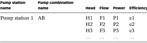
After calculation of all parameters of sample points in the pump combination characteristic curves, the results will be stored in database in the format shown in Table 2.
Optimization method
In the case of multi-objective optimization, instead of obtaining a unique optimal solution, a set of equally good (non-dominating) optimal solutions is usually obtained (Pareto sets). Several methods, such as meta-heuristic algorithm (Kim et al. ), versions of GA (Khu & Keedwell ; Alvisi and Franchini ), NSGA-II (Deb et al. ) and particle swarm optimiz-ation algorithm (Liu et al. ) are available to solve multi-objective optimization problems. NSGA-II is used here to obtain the Pareto set.
Coding and decoding
Since only the head of elevated reservoirs are decision vari-ables, so the number of genes in chromosomes is equal to the number of reservoirs. Because different reservoirs may have different head ranges, each reservoir’s head range is discretized into n points by equal intervals, so that the gene code of each reservoir can be coded from a uniform integer gene code pool which is composed of integers from 0 ton, and the searching space becomes smaller. The chromosome string can be represented by an integer array, and each element of the integer array stores a gene code of the chromosome string, and each gene code belongs to the set of (0, 1, 2…,n). The decoding process is to calculate the head of each reservoir from the gene code, and can be expressed by Equation (6):
Hi¼Himinþ(HimaxHimin)
gi
n (6)
wheregiis theith gene code in the chromosome,Hiis the
head of the ith reservoir calculated from gi, Himin and
Himaxis low and up boundary of the head of theith
reser-voir,nis the size of the gene code pool.
Calculation of individual’s objective values andfitness
In the evolving process, the three objective values of each solution are obtained in different levels. In the first opti-mal level, by decoding chromosome string into reservoirs’ water level and by hydraulic simulation, the objective value of lower pressure service nodes amount can be obtained. Since the outflow of each reservoir is calculated in hydraulic simulation, so the optimal pump combination for each reservoir can be selected from the pump combination database according to outflow, head and neighbourhood region. After the pump combination is selected, the electricity cost objective value and error objective value can be calculated. The pump combi-nations of the simulated period are determined. The pump combinations will be stored in the individual of each solution. After calculation of objective values, sol-utions will be sorted by a non-dominated sorting method, and assigned rank value.
Table 2|The example records of pump combination scheme database
Pump station name
Pump combination
name Head Flow Power Efficiency
Pump station 1 AB H1 F1 P1 e1
H2 F2 P2 e2
H3 F3 P3 e3
Genetic operations
The roulette wheel selection, one point crossover and real valued mutation are used in GA operation of this study. For optimization problems, the termination condition is also an important aspect that impacts the algorithm’s per-formance. In traditional ways, errors between the last iterations’results can be used as the termination condition. For example, when the error between the last two iter-ations’ results is less then a designated value then the iteration stops. However, for GAs these kinds of termin-ation conditions may cause a premature termintermin-ation
when GA converges to a local optimal solution. So assig-ment of a large generation number is a popular method of termination condition in GAs, and this method is used in the proposed merged two-level optimal method. The whole optimal methodology framework is shown in Figure 3.
The pump operation schedules of each reservoir in the simulated period will be obtained after a run of the merged two-level optimal method. For an extended period of pump schedules operation, the merged two-level optimal method should be run several times equal to time steps in total duration.
CASE STUDY
A real WDS in North China is used here as a case study net-work. This WDS serves a population of nearly 3 million. Daily water consumption is in the range of 0.7–0.9 million m3. In the daily water consumption pattern, there are two consumption peaks, generally at 10 am and 7 pm. The studied WDS has seven pump stations (each pump station has a reservoir) and 48 pumps. In total, the network consists of 3732 nodes and 4522 links with a total length of 764.76 km. Details of the pump stations are shown in Table 3.
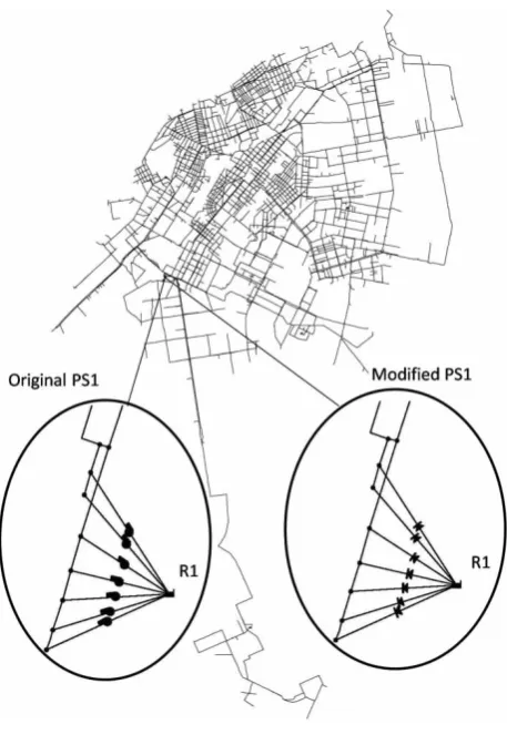
Before running of the merged two-level optimal method, the hydraulic model needs to be modified. The modification method is replacing pump links which con-nect reservoirs with pipe network by pipe links with a check valve. Figure 4 shows the layout of the network. PS1 is used as an example to show the modifications to the pump stations. In this case, a typical 24 h scheduling period is used to test optimal methodology, and the period is divided into 24 1-hour simulation steps. So the merged two-level optimal model solved by NSGA-II will run 24 times obtain pump schedules for the typical 24 h period. In order to evaluate the average performance of the merged two-level optimal model, 10 runs of 24 h pump scheduling optimization were conducted using differ-ent random seeds. Each run is executed with the same GA parameters setting: population size is 100, generation size is 100, crossover probability is 0.6 and mutation probability is 0.1.
RESULTS AND DISCUSSION
Since the pump schedules result is obtained by an enumer-ation algorithm with a pump combinenumer-ation database and modified hydraulic model, the optimal result should be examined by the original hydraulic model with a run accord-ing to the optimal pump schedules results. Only when simulation results of the original model and the modified model are met can the feasibility of the merged two-level optimal methodology based on the pump combination data-base and the modified hydraulic model be guaranteed. A comparison between hydraulic simulation results of total outflow from each reservoir of the two hydraulic models is shown inTable 4. There are 10 runs of 24 h pump schedul-ing optimization, so the maximum, minimum and average values of errors between two models are shown inTable 4. The values inTable 4are relative errors that were calculated
Figure 4|Layout of network.
Table 3|Information of pump stations
Name
Reservoir name and head boundaries
(m) Pump type and count
PS1 R1 (20–60) 12sh-9(7)
PS2 R2 (20–60) 20LN-26A(7), 12LN-21B
(3)
PS3 R3 (20–70) S500-59(5), 500S-98B(2)
PS4 R4 (20–60) 12sh-9(4), 14sh-13A(1)
PS5 R5 (20–60) 24SA-10A(3), 16SA-9C
(3)
PS6 R6 (10–60) 12sh-13(4), 12sh-9A(2)
by Equation (7):
error¼jr0rmj
r0 (7)
wherer0is the simulation result of the original model, and
rmis the simulation result of the modified model.
InTable 4the maximum relative error of the two models is less than 0.05. It shows that there is little error between the hydraulic simulation results of the two models. So it is feasible to use a modified model and pump combination database for calculation of objective values in the optimal process as a surrogate of the original hydraulic model.
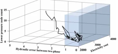
Figure 5shows the 3D line which represents the conver-gence path of the evolution process. Each junction of the 3D line represents the average objective values of one gener-ation. The objective value of‘hydraulic error between two optimal levels’has been processed, the integer part of objec-tive value represents the number of reservoirs without a feasible pump combination, and the fraction part represents the relative hydraulic error.
FromFigure 5it can been seen that the hydraulic error objective converges to the feasible solution space rapidly and searches for better solutions in the feasible solution space. The transparent blue box defines the feasible solution space. In this space, the objective value of‘hydraulic error between two optimal levels’is less than 1. This means that
solutions found in this space all have feasible pump combi-nations for every reservior of WDS. Generally, after 30–40 generations evolution the average objective values can enter the feasible solution space, and use the rest of the evol-ving process to search the feasible solution space thoroughly. If considering the best solutions generated during the evolving process, some best solutions reach the feasible solution space much earlier than the average sol-utions, so the search process in the feasible solution space should start much earlier than the situation shown in Figure 5. This performance is a result of merged two-level optimization. By embedding the second optimal level into the first optimal level, the solutions without a feasible pump combination and solutions with poor hydraulic per-formances are eliminated in the initial generations of the evolving process, and lead the search direction to the feas-ible solution space. This prevents the possibility of generating unfeasible results in the whole optimal process.
The second concern is the quality of the optimal result. The quality of the optimal result can be evaluated from two aspects: electricity cost and hydraulic performance of WDS. A comparison between the optimized optimal pump sche-dules and the original pump schedule from the aspect of electricity cost is shown inTable 5.
The original pump schedule is used in the case study WDS in the summer water consumption pattern, and is cor-rected by years of running experience. With years of correction it is nearly perfect and has little scope to be opti-mized by experience. Finding better pump schedules for the case study WDS is a challange of the proposed optimization method. FromTable 5 it can be seen that each run of the optimal method finds a lower electricity cost pump sche-dule, and the average reduction of electricity cost is more than 5%. So the proposed method has the ability tofind a better pump schedule for WDS’s electricity cost reduction. Figure 6shows the electricity cost reduction of 10 runs of the two-level optimal method.
Table 4|Comparison between total outflow from each reservoir of the two hydraulic models
R1 R 2 R 3 R 4 R 5 R 6 R 7
Max error 0.021 0.016 0.030 0.048 0.019 0.022 0.029
Min error 0.005 0 0.001 0.003 0.001 0.002 0.002
Average error 0.012 0.004 0.011 0.023 0.009 0.011 0.016
The solid line and dashed line express the maximum and minimum electricity cost reduction among 10 runs. The area between the two lines is the band that represents the electricity cost potentiality found by the merged two-level optimization. Most of the band area is above the abscissa axis, it means in most cases the optimal method found pump combinations with lower electricity cost. For the case network, most cost reductions were achieved at night. This indicates that the original pump schedule for the night hours has room for improvement.
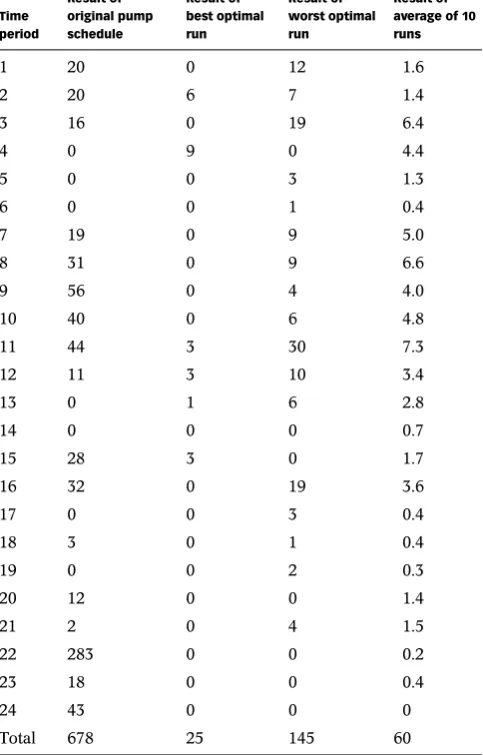
Table 6shows the comparison of lower service pressure nodes between the original pump schedule and the optimal pump schedules.
It can be seen from Table 6 that lower service head nodes in the test network with optimal pump schedules are much less than the situation with the original pump schedule. It shows that the proposed method has the ability tofind solutions which not only reduce the electricity cost but also enhance the hydraulic performance of WDS. By transforming the lower service pressure constraint into an objective function in the optimal process, better solutions in both cost saving and hydraulic performance enhance-ment were found. Since there are no penalty functions or weighted coefficients used in the optimal process, the
unreasonable setting of penalty functions or weighted coeffi-cients is avoided. This makes the merged two-level optimal method a robust method in finding better solutions of lower cost and high hydraulic performance.
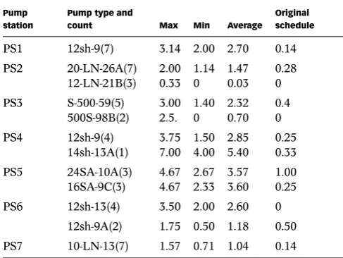
One thing that should be considered but is not discussed in this study is pump ON/OFF switch times. Because the optim-ization for each 1-hour simulation step is implement isolated, so the pump switch times during the 24 h pump scheduling optimization could not be concerned in the optimal process. Table 7shows the average times of each pump type in the pump stations. Since the optimal result is shown in the format of pump combination with pump type and its number for each pump station, the optimal result does not give the operation schedule for each pump, so the average times of
Figure 6|Electricity cost reduction. Table 5|Summary of electricity cost reduction
Electricity cost of original pump schedule (¥¥)
Electricity cost of optimal pump schedule (¥¥)
Reduction ratio
86308 Best 79893 0.071
Average 81262 0.056
Worst 82461 0.042
Table 6|Comparison of lower service pressure nodes
Time period
Result of original pump schedule
Result of best optimal run
Result of worst optimal run
Result of average of 10 runs
1 20 0 12 1.6
2 20 6 7 1.4
3 16 0 19 6.4
4 0 9 0 4.4
5 0 0 3 1.3
6 0 0 1 0.4
7 19 0 9 5.0
8 31 0 9 6.6
9 56 0 4 4.0
10 40 0 6 4.8
11 44 3 30 7.3
12 11 3 10 3.4
13 0 1 6 2.8
14 0 0 0 0.7
15 28 3 0 1.7
16 32 0 19 3.6
17 0 0 3 0.4
18 3 0 1 0.4
19 0 0 2 0.3
20 12 0 0 1.4
21 2 0 4 1.5
22 283 0 0 0.2
23 18 0 0 0.4
24 43 0 0 0
each pump type in the pump station is used here to evaluate pump switch times. Average times of each pump type is calcu-lated by dividing total switch times of certain pump type by pump number of that pump type. There are 10 runs of optimal method, and the maximum, minimum and average values of
‘average switch times of each pump type’ is shown in
Table 7, and the average pump switch times of original pump schedule are also shown as a comparison.
FromTable 7it can be seen that the pump switch times of optimal result is obviously higher than switch times in the original pump schedule. A reasonable explanation for the increase of pump switch times is that to meet the objective of electricity cost reduction, the selected pump combination for each 1-hour simulation step should meet the water con-sumption in WDSs more precisely, so that running pumps can stay in a high efficiency state, however, this can also cause a situation of high frequency of ON/OFF switches of pumps. So when consumption demand changes the pump combination tries tofind a high efficiency pump combination to attain the minimum electricity cost objective. The impor-tant thing is that the pump switch times should stay in an acceptable range. Since there is no tradeoff between electri-city cost reduction and pump switch times, so the result of high pump switch times occurred in the proposed method-ology. Although the pump switch times are higher than the original pump schedule, the optimal schedules of most pump stations are acceptable. The maximum number of sim-ultaneously running pumps in each pump station in the
WDSs is set as 4, so certain pump types with spare pumps have a relatively lower average pump switch time because the total switch times can be shared by relatively more pumps, for example, there are seven pumps of type 10-LN-13 in PS7, and the maximum pump switch times of this type is 11 during a whole 24 h pump schedule period. Divided by seven, each pump only experienced 1.57 ON/OFF occur-rences in 1 day. An extreme case of high switches is the pump of 14sh-13A in PS4, because there is only one pump of that type in the pump station, so all switches will act on this pump. In this case, an operation schedule modification for certain pumps should be carried out manually.
The computational effort required by the merged two-level optimal method was measured when run on a Core 2 Duo T6500 (2.10 GHz) with 2048 kb of cache size running under Windows XP. The mean computation time required for one run of one hydraulic simulation step of the case network was 1198 s, while it was 7.99 hours for a 24 h pump schedules optimization with a hydraulic step of 1 h. Since each optimal process for every simulation step is run totally separately, the total computation time can be shortened by parallel runs of optimal program in one computer or several computers.
CONCLUSIONS
By introduction of a hydraulic model and pump combination database, a merged two-level optimal method for WDS optimal pump operation is proposed. By transforming the pump station of the original hydraulic model into an elevated reservoir, the modified model can be used in thefirst optimal level for evalu-ation of hydraulic performance of candidate solutions, and the defects of fallibility and incomplete hydraulic performance evaluation of meta-model are avoided and more reliable sol-utions can be obtained. By building a pump combination database, the enumeration algorithm is used in the second opti-mal level, and the complexity of second optiopti-mal level is reduced significantly. This makes it possible to run the second optimal level process to each solution in each evolving step of evolution algorithms, so that the second optimal level can be embedded into thefirst optimal level to form a merged two-level optimal methodology. Be embedding the second optimal level into thefirst optimal level, the solutions without a feasible pump combination will be eliminated and lead the solving process
Table 7|Pump switch times result
Pump station
Pump type and
count Max Min Average Original schedule
PS1 12sh-9(7) 3.14 2.00 2.70 0.14
PS2 20-LN-26A(7) 2.00 1.14 1.47 0.28
12-LN-21B(3) 0.33 0 0.03 0
PS3 S-500-59(5) 3.00 1.40 2.32 0.4
500S-98B(2) 2.5. 0 0.70 0
PS4 12sh-9(4) 3.75 1.50 2.85 0.25
14sh-13A(1) 7.00 4.00 5.40 0.33
PS5 24SA-10A(3) 4.67 2.67 3.57 1.00
16SA-9C(3) 4.67 2.33 3.60 0.25
PS6 12sh-13(4) 3.50 2.00 2.60 0
12sh-9A(2) 1.75 0.50 1.18 0.50
to converge on the feasible solution space so that a generation of impracticable results can be avoided. A multi-objective opti-mal model and solving method NSGA-II are used in this study, hydraulic constraint of lower service node count and hydraulic errors between two levels are regarded as objectives in parallel with electricity cost objective in the multi-objective model. These measures solve the problems of unreasonable penalty functions or the setting of weighted coefficients that occur in optimization methods using single objective optimal models.
Since there is no limitation for maximum pump switch times in the optimal process, sometimes results with a high frequency of pump switches will be obtained by the proposed method. In this case, a manual modification to optimal results should be carried out before pump schedules are put into effect.
ACKNOWLEDGEMENTS
The authors acknowledge the support from Seventh Framework Programme (FP7) Marie Curie Actions International Research Staff Exchange Scheme- Smart Water (PIRSES-GA-2012-318985) and FP7-WatERP (EC-318603), and also acknowledge the support from the Project of Construction Science and Technology-Component Based Software Development of Information Management Platform of Water Distribution System (2010-53).
REFERENCES
Alvisi, S. & Franchini, M.Near-optimal rehabilitation scheduling
of water distribution systems based on a multi-objective genetic algorithm.Civil Eng. Environ. Syst.23(3), 143–160.
Bagirov, A. M., Barton, A. F., Mala-Jetmarova, H., Al Nuaimat, A.,
Ahmed, S. T., Sultanova, N. & Yearwood, J.A novel
approach to optimal pump scheduling in water distribution
systems. In:14th Water Distribution Systems Analysis
Conference, Adelaide, South Australia, pp. 618–631.
Benjamín, B., von Christian, L. & Aldo, S.Multi-objective
pump scheduling optimisation using evolutionary strategies. Adv. Eng. Softw.36(1), 39–47.
Boulos, P. F., Zheng, W., Chun, H. O., Michael, M., Paul, H. &
Devan, T.Optimal pump operation of water distribution
systems using genetic algorithms. In:Proc., Distribution
System Symp., AWWA, San Diego, pp. 23–25.
Deb, K., Pratap, A., Agarwal, S. & Meyarivan, T.Fast and
elitist multi-objective Genetic Algorithms: NSGA-II.IEEE Trans. Evol. Comput.6(2), 182–197.
Fang, H., Wu, W., Lv, M. & Gao, J.Optimising pump system
with constant and variable speed pumps: case study.Int. J. Modell. Ident. Control12(4), 412–420.
Kevin, E. L. & Kofi, A.Optimal pump operation considering
pump switches.J. Water Resour. Plann. Manage. ASCE120 (1), 17–35.
Khu, S. T. & Keedwell, E.Introducing more choices (flexibility)
in the upgrading of water distribution networks: the New York city tunnel network example.Eng. Optimiz.37(3), 291–305.
Kim, J. H., Baek, C. W., Jo, D. J., Kim, E. S. & Park, M. J.
Optimal planning model for rehabilitation of water networks. Water Sci. Technol. Water Supply4(3), 133–147.
Liu, D. S., Tan, K. C., Huang, S. Y., Goh, C. K. & Ho, W. K.On
solving multi-objective bin packing problems using evolutionary particle swarm optimization.Eur. J. Operat. Res.190(2), 357–382.
López-Ibáñez, M., Prasad, T. D. & Paechter, B.Ant colony
optimization for optimal control of pumps in water distribution networks.J. Water Resour. Plann. Manage.134(4), 337–346.
Mackle, G., Savic, D. A. & Walters, G. A.Application of genetic
algorithms to pump scheduling for water supply. In:Proc.,
Genetic Algorithms in Engineering Systems: Innovations and Applications, GALESIA’95, IEEE, Sheffield, UK, pp. 400–405.
Ormsbee, L. & Lansey, K.Optimal control of water supply
pumping systems.J. Water Resour. Plann. Manage.120, 237–252.
Ormsbee, L., Walski, T., Chase, D. V. & Sharp, W. W.
Methodology for improving pump operation efficiency.J. Water Resour. Plann. Manage.115(2), 148–164.
Price, E. & Ostfeld, A.Iterative linearization scheme for
convex nonlinear equations: application to optimal operation of water distribution systems.J. Water Resour. Plann. Manage.139(3), 299–312.
Savic, D. A., Walters, G. A. & Schawb, M.Multi-objective
Genetic Algorithms for Pump Scheduling in Water Supply. ERASMUS, Exeter, UK/Stuttgart, Germany: School of Engineering of Exeter University/University of Stuttgart.
Van Dijk, M., Van Vuuren, S. & Van Zyl, J.Optimising water
distribution systems using a weighted penalty in a genetic
algorithm.Water SA34(5), 537–548.
Yuan, Y. X., Zhong, D. & Gao, J. L.Optimization operation
of water distribution system based on macroscopic model. China Water Wastewater26(5), 55–62.
Zhang, T. Q., Lv, M. & Zhao, H. B.Research into optimal
control algorithms in water-supply networks.J. Zhejiang Uni.
(Eng. Sci.)34(4), 428–432.
Zheng, S. Y.Study on the macroscopic model of two-grade
optimization operation in urban water supply system. J. Sichuan Union Uni. (Eng. Sci. Edn.)1(2), 60–68.