Facial Expression Recognition with Fusion Features Extracted from Salient Facial Areas

Facial Expression Recognition with Fusion Features

Extracted from Salient Facial Areas

Yanpeng Liu, Yibin Li, Xin Ma, Rui Song *

SchoolofControlScienceandEngineering,ShandongUniversity,Jinan 250061,China * Correspondence: [email protected]

Abstract: In pattern recognition domain, deep architectures are widely used nowadays and they have achieved fine grades. However, these deep architectures need special demands, especially big datasets and GPU. Aiming to gain better grades without deep networks, we propose a simplified algorithm framework using fusion features extracted from the salient areas of faces. Furthermore, the proposed algorithm has achieved a better result than some deep architectures. For extracting more effective features, this paper firstly defines the salient areas on the faces. This paper normalizes the salient areas of the same location in the faces to the same size, therefore it can gain more similar features from different subjects. LBP and HOG features are extracted from the salient areas, fusion features’ dimensions are reduced by Principal Component Analysis( PCA) and we apply softmax to classify the six basic expressions at once. This paper proposes a salient areas definitude method which uses peak expressions frames to compare with their neutral faces. This paper also proposes and applies the idea of normalizing the salient areas to align the specific areas which express the different expressions. This makes the salient areas found from different subjects have the same size. Besides, gamma correction method is firstly applied on LBP features in our algorithm framework which improves our recognition rates significantly. By applying this algorithm framework, our research has gained state-of-the-art performances on CK+ database and JAFFE database.

Keywords: facial expression recognition; fusion features; salient facial areas; hand-crafted features; feature correction

1. Introduction

Facial expression plays an important role in our daily communication with other people. For the developing of intelligent robots, especially the indoor mobile robots, emotional interactions between robots and human are the foundational functions of these intelligent robots. Facial expression recognition is an important part of human-robotics interaction technology. Many research works have been done in the literature, the universal expressions mentioned in papers are usually anger, disgust, fear, happiness, sadness and surprise [1–3] while some researchers add neutral and contempt [4,5].

2 of 17

recognition domain. AU-inspired Deep Networks (AUDN)[2], Deep Belief Networks (DBN)[10] and Convolutional Neural Network (CNN) [6,11] are used in the facial expressions recognition work. Apart from the higher recognition rate, more computing resources and data are needed in these algorithms. For these reasons, the former framework is applied in our research.

Face alignment is applied to help researchers to extract more effective features from the static images[4,12]. Automated facial landmark detection is the first step to complete this work. After finding these landmarks on the faces, researchers can align the faces and extract features from these faces. Early days, researchers only use fewer landmarks to align the faces and separate the faces to several small patches for extracting features [9]. This can roughly alignment the faces while more landmarks can improve the alignment precision. There are many methods to detect landmarks from the faces. Tzimiropoulos et al.[13] have proposed a Fast-SIC method for fitting AAMs to detect marks on the faces. Zhu [14] et al. use a model based on the mixture of trees with a shared pool marks 68 landmarks on the face. This method is applied in our algorithm and 68 landmarks are used to align the salient areas. These landmarks mark the shape of eyebrows, eyes, nose, mouth and the whole face, which can help researchers to cut the salient patches. Although alignment faces can help to extract more effective features from the faces, some areas on the faces do not align well during this process. In this paper, the idea of normalizing the salient areas is firstly proposed to improve the features extracted effectiveness.

In order to reduce the features’ dimensions and extract more effective features, different salient areas definitude methods are proposed in literatures. Zhong et al.[3] explained the idea that discovering the common patches across all the expressions is actually equivalent to learning the shared discriminative patches for all the expressions in their paper. They transferred the problem into a Multi-task sparse learning (MTSL) problem and by using this method they had gained a good result. Happy et al.[9] applied these areas found in their paper and they also gained a decent result. Liu et al.[2] used Micro-Action-Pattern Representation in the AU-inspired deep networks (AUDN) and built four criterions to construct the receptive fields. This gained a better result and accomplished the features extraction at the same time. In order to define the salient areas more accurately, our research uses the neutral faces to compare with the peak frames of these expressions. Karl Pearson correlation coefficient[15] is applied to evaluate the correlation between the neutral faces and the faces expressed different expressions. For finding the precise locations of the salient areas, the faces are separated to several small patches. After comparing the small patches to their neutral faces, the patches which have weaker correlation coefficient are found and these are the areas expressing the specific expression. By using this method, the salient areas of the six fundamental expressions are found and after fusing these areas the salient areas of the six basic expressions are found too. Landmarks of the faces are used to locate these salient areas and different size of salient areas are normalized in our research framework.

Different kinds of descriptors are applied in facial expressions recognition research. Regarding the scale of the features extracted areas, the hand-crafted features are extracted from the whole alignment face in the earlier time [4,12] while the salient areas are used in hand-crafted extraction in nowadays [3,9]. Aiming to describe the different expressions more effectively, diverse features extracted methods are used in facial expression recognition. Typical hand-crafted features include Local Binary Patterns (LBP) [4],Histogram of Oriented Gradient (HOG) [8], Scale Invariant Feature Transform (SIFT) [16], and the fusion of these features [7]. According to these literature, the fusion features contain more information about these expressions and achieve better results. That is the reason why we chose to extract LBP and HOG from the faces. Although fusion features can improve recognition rate, it is hard to fuse these features well. Before different features fuse together, normalization methods are applied to the features. Although utilizing this normalization method can improve the recognition result, different kinds of features’ identities cannot mix well. Aiming to use more information of the LBP features and normalize the LBP features, gamma feature correction method is firstly applied on LBP features in our algorithm frameworks.

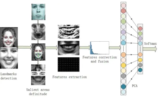
Figure 1.Framework of the proposed algorithm.

In this paper, we have proposed a straightforward but effective algorithm framework to recognize the six basic expressions from static images. By comparing the neutral faces to these expressions, the salient areas are defined. The salient areas are separated from the faces according to these landmarks on these faces. The idea of normalizing the salient areas is firstly proposed to overcome salient areas misalignment. After finishing that, we extract LBP and HOG features from the areas and fuse the features. Before applying softmax to classify the six expressions, Principal Component Analysis( PCA) is utilized to reduce the dimensions. Our algorithm framework is shown in Fig. 1. By using this framework, we have gained a better grade than the deep networks [2,10].

2. Methodology

In this section, the proposed algorithm will be explained in details. This section will focus on the salient facial areas definitude principle introduction and show the salient areas normalization and features fusion methods. LBP features correction methods will be introduced and applied in our algorithm. Apart from that these other modules of our paper will be simply and clearly introduced too.

2.1. Faces Alignment and Salient Facial Areas Definitude

Automated facial landmark detection is the first step in our method. Facial landmark detection is an important basement for facial expression classification. The method that applied in the paper [14] is chosen to mark 68 landmarks on the faces in our research. These landmarks mark the shape of eyebrows, eyes, nose, mouth and the whole face, so these specific areas can be located by these landmarks. These 68 landmarks on the face and the normalized face have been shown in Fig. 1. According to the average length and width of the faces and the proportion of the length and width, the faces in CK+ database are normalized to 240x200.

4 of 17

Figure 2.The salient areas of the 6 expressions. (a) Salient areas of all expressions and the neutral.(b) Salient areas of anger. (c) Salient areas of disgust. (d) Salient areas of fear. (e) Salient areas of happy. (f) Salient areas of sad.(g) Salient areas of surprise.

method and gain a good result. In order to learn expression specific features automatically, Liu et al. [2] proposed an AU-inspired deep network (AUDN). They used Micro-Action-Pattern Representation in the AUDN and built four criterions to construct the receptive fields. This gained a better result and accomplished the features extraction at the same time.

These methods all found salient areas from the aligned faces and extracted features from these salient areas. As for our algorithm, the areas which are more salient to their own neutral faces are found firstly. In the last paragraph, the 68 landmarks have been found and the faces are normalized to 240x200. The areas in the six basic expressions are compared to their neutral faces at the same location. If the areas during the expressions have not moved around, the areas must be more correlation with the areas on their neutral faces. Using this principle, comparing to the other correlation coefficient methods in [15] Karl Pearson correlation coefficient is applied to evaluate the correlation between the neutral faces and the faces expressed different expressions. Karl Pearson correlation coefficient is applied to evaluate the correlation between the matrixes. For finding the precise locations of the salient areas, the faces are separated to 750 (30x25) patches and every patch is 8x8 pixels. These 8x8 pixels patches are matrixes and by comparing the small patches from neutral faces and specific expressions, the salient areas can be found precisely. Karl Pearson correlation coefficient formulate is shown next.

γ_ijk = ∑m(Em−

¯

E)(Nm−N¯) p

(∑m(Em−E¯)2)(∑m(Nm−N¯)2)

(1)

Whereγk_ijis the(i,j)th patch’s correlation coefficient of specific expressions, so the scale ofiis 1 to 30, jis 1 to 25.

Rij =

∑

ρk∗γ_ijk (2)

In order to find the salient areas of all these six basic expressions, a formula is defined to evaluate the final correlation coefficient. TheRijis the final correlation coefficient of the (i,j)th location on face. By changing theρk, the different proportion of thekth expression can be changed. Besides, the sum of theρkmust equal to 1.

6

∑

ρk=1 (3)

The results of the six expressions are shown in the Fig. 2. These areas found in this section will be applied in the next section. From the Fig.2, we can find that different expressions have different salient areas. Equation(1) is used to evaluate the salient areas in the six fundamental expressions. In equation(3),ρkexpresses the proportion of the specific expression in the final result, the value ofρk can be changed according to the recognition rate.

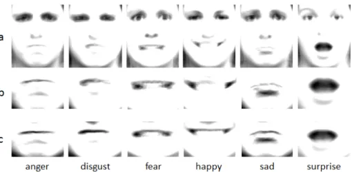
Figure 3. Average faces and the average salient areas. (a) Average faces of the six expressions.(b) Mouth parts of the average faces. (c)Average salient mouth areas.

2.2. Salient Areas Normalization and Features Extraction

In this section, an idea of normalizing the salient areas rather than the whole faces is proposed and applied. Furthermore, local binary patterns (LBP) features and the histogram of oriented gradient (HOG) features all are extracted from the salient areas. Comparing to the method extracting features from the whole faces, features extracted from salient areas can reduce the dimensions, lower noise impacts and avoid overfitting.

2.2.1. Salient Areas Normalization

In the last section, the salient areas are found out. Our research has a similar result as the result in [3], but there have different performance in the eyes parts. In papers [3,9], the researchers used the patches of the faces which come from alignment faces. Normalizing the whole faces is a good idea before more landmarks can the marked from the faces. Now more landmarks can be marked from the faces, this makes it easier to extract the salient areas from the faces. There are two main reasons for choosing to normalize the salient areas.

Firstly, aligning the faces may result in salient areas misaligned. In order to demonstrate the alignment effects, the faces are aligned and then all the faces in one specific expression are added to gain the average face. The each pixelXijis the average of all images of the specific expression.

Xij= 1

n

∑

6 of 17

Figure 4. (a)Calculation progress of the original LBP value. (b) Mouth area and the Pixels is 40x60. (c)Mouth area and the former pixels is 28x42, the real pixels is enlarged from the former image .(d) Display models of (b) and (c) mouth.

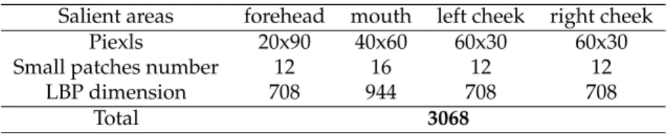
Table 1. Patches numbers and LBP dimensions of salient areas

Salient areas forehead mouth left cheek right cheek

Piexls 20x90 40x60 60x30 60x30

Small patches number 12 16 12 12

LBP dimension 708 944 708 708

Total 3068

areas alignment. In the experiment section, comparative experiments will be designed to compare the effects of the salient areas alignment method with the traditional faces alignment methods.

2.2.2. Features Extraction

• Local Binary Patterns (LBP)

Texture information is an important descriptor for pattern analysis of images, and local binary patterns (LBP) was presented to gain texture information from the images. LBP was first described in 1994 [18,19] and from then on LBP has been found to be a powerful feature for texture representation. As for these facial expressions, actions of the muscles on the faces lead the faces to generate different textures. LBP features can describe the texture information of the images and this is the reason why LBP features are extracted from the salient areas. The calculation progress of the original LBP value is shown in Fig. 4(a). A useful extension to the original operator is the so-called uniform pattern [20], which can be used to reduce the length of the feature vector and implement a simple rotation invariant descriptor. In our research, uniform pattern LBP descriptor is applied to gain features from the salient areas, and the salient areas are all separated to small patches. LBP features are gained from these salient areas respectively and these features are concatenated as the final LBP features. The length of the feature vector for a single cell can be reduced from 256 to 59 by using uniform patterns. This is very important, for there are many small patches in our algorithm. For example, the size of the mouth area is 40x60 and the small patches’size is 10x15, so the mouth area is divided into 16(4x4) patches. The uniform LBP features are extracted from each small patch and mapped to a 59-dimensional histogram. The salient areas all are separated into several small patches and the results are shown in Fig. 5. The numbers are shown in Table 1. The dimension of the final LBP features is 3068 by adding these numbers in Table 1.

Figure 5.Small patches of salient areas. (a) Mouth areas, anger, fear, happy.(b) Forehead areas, anger, fear. (c)Cheek areas, left cheek fear, right cheek fear, left cheek anger, left cheek happy, right cheek happy.

Table 2. Patches numbers and HOG dimensions of salient areas

Salient areas forehead mouth left cheek right cheek

Piexls 20x90 40x60 60x30 60x30

Small patches number 51 77 55 55

HOG dimension 1836 2772 1980 1980

Total 8568

For different features will be extracted from different size of salient areas, these salient areas should be aligned. In order to demonstrate the difference, different sizes of mouth areas are cut from one face and these areas are normalized to the same size. These mouth areas are shown in Fig. 4. LBP features are extracted from these normalized faces and their distributions are shown in Fig. 4. From the figure, a conclusion can be drawn that different size of images have different LBP features. The values’ number in (d) and (e) have different performance. Besides, HOG features also are extracted from these salient areas, they have the similar result as LBP features.

• Histogram of Oriented Gradient (HOG)

8 of 17

Figure 6.HOG descriptors of the mouths. (a) Happy mouth areas.(b) Fear mouth areas.

2.3. Features Correction and Features Fusion

2.3.1. LBP Correction

LBP feature is a very effective descriptor of the texture information of images. Many researchers [3,9] applied LBP to describe these different expressions. In our algorithm, LBP features are extracted and processed before they are sent into the classifiers. For most papers, researchers extract features from images and normalize the data to 0-1, such as [23] normalizes the data to 0-1. For our algorithm framework, the images data are normalized to 0-1, by using this method a better result can be gained. In order to normalize the LBP features of every subject, the method in equation(5) is applied to normalize the LBP features to 0-1.

Lm= lm

max(lm) (5)

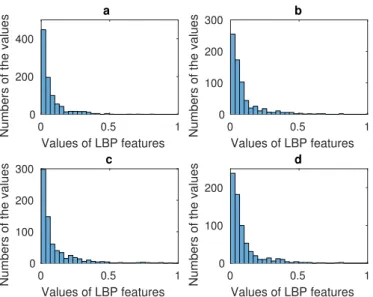
wheremis the dimension number of every salient area. Aiming to utilize the specific characteristic of every area, the four salient areas are normalized respectively. The distribution styles of these LBP features extracted from the four salient areas are displayed in Fig. 7. The figure shows that the distribution model of LBP features is power law distribution. In images processing, gamma correction redistributes native camera tonal levels into ones which are more perceptually uniform, thereby making the most efficient use of a given bit depth. In our algorithm, the distribution of LBP features is power law distribution, for using more information and making it easy to fuse LBP and HOG features, gamma correction is used to correct the LBP feature data.

¯ Lm=L

1 λ

m (6)

whereλis the correct gamma number. As we all know, most numbers of gamma number came from experiment experience data. An evaluation method to find the proper gamma value is proposed in our algorithm.

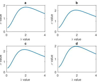
For the power law distribution, fewer data contain more information. In order to use more information of LBP features, gamma correction method is chosen to process the LBP features and σis applied to get the proper gamma number for every salient area. Every salient area is processed respectively, so fourσvalues will be gained. The relationships between these four salient areas’σand the gamma numberλare shown in Fig. 8. According to the experimental data, all the four salient

0 0.5 1 Values of LBP features 0

200 400

Numbers of the values

a

0 0.5 1

Values of LBP features 0

100 200 300

Numbers of the values

b

0 0.5 1

Values of LBP features 0

100 200 300

Numbers of the values

c

0 0.5 1

Values of LBP features 0

100 200

Numbers of the values

d

Figure 7.(a) Display model of mouth’s LBP features.(b) Display model of left cheek’s LBP features.(c) Display model of forehead’s LBP features. (d) Display model of right cheek’s LBP features.

areas have the maximumσvalue aroundλ’s value 2. Therefore, all the four salient areas’σvalue are added to find the final sum and the relatedλ.

σ= 1

np

∑

∑

2 ₍₇₎

Un= 1

p

∑

Wherenis the number of the images’ number,pis the number of nonzero data in LBP features of the salient areas. Therefore,pis smaller than the dimensions of the salient areas’ LBP features. Unis the mean of the specific subjects. In our algorithm, the relationship between theσ, gamma numberλand the recognition rate have been found, and the relationship is shown in Fig 9.

2.3.2. HOG Processing and Features Fusion

Different features describe different characters of the images, therefore researchers used some features merging together to apply the superiority of all the features [9,23]. For our algorithm, LBP and HOG descriptors are applied to utilize the texture and oritension information of these expressions. Proper fusion methods are very important factors for the recognition work and uncomfortable methods can make the recognition result worse. The recognition rate of the individual feature and fusion features will be shown in the experiment section. Zhang et al. [23] applied a structured regularization(SR) method which is employed to enforce and learn the modality specific sparsity and density of each modality respectively. As for our algorithm, the single features are firstly processed to their best performance and then they are normalized to the same scale. In the experiment section, different experiments are proposed to explain the results of single features and the fusion feature.

Gamma correction method is applied to make the LBP reach their best performance. Different features must be processed to the same scale when these features are fused together. The Z-score method is used to process LBP and HOG features, and after applying the method the average is 0 while the variance is 1.

σ=

J

∑

j

10 of 17

0 2 4

λ value 0

1 2

σ

value

a

0 2 4

λ value 0

1 2

σ

value

b

0 2 4

λ value 0

1 2

σ

value

c

0 2 4

λ value 0

1 2

σ

value

d

Figure 8.(a) Relationship between mouth’sλandσ.(b) Relationship between left cheek’sλandσ.(c) Relationship between forehead’sλandσ. (d) Relationship between right cheek’sλandσ.

µ=

∑Jj fj

J (10)

ˆ fj =K

(xj−µ)

σ+C (11)

Where fjis the data of LBP or HOG feature and ˆfj is the feature data after processing. As for LBP features, although the display model has changed, the data changing to the same scale and a better result can be gained. Because ˆfjis too small, numberKis used to multiply ˆfj. In our experiment, the

Kequal to 100.

2.4. Principal Component Analysis( PCA) and Softmax Regression Classifier

Principal Component Analysis (PCA) was invented in 1901 by Karl Pearson [24] as an analog of the principal axis theorem in mechanics, it was later independently developed by Harold Hotelling in the 1930s [25]. Principal component analysis (PCA) is a statistical procedure that uses an orthogonal transformation to convert a set of observations of possibly correlated variables into a set of values of linearly uncorrelated variables called principal components. PCA is an effective method to reduce the features dimension, there are many researchers using this method to reduce the features’ dimension. In our algorithm, the fusion features’ dimension is 11636, and it is really a huge number. In order to reduce the feature’s dimension, PCA is applied to reduce the dimension to a proper number. The relationship between the recognition date and the number of the dimension is shown in Fig. 10. According to the experiment, the most proper dimension is 80.

Softmax regression is a generalization of logistic regression to classify multiple classes, and this means that softmax can be used to classify many classes in once time. In neural network framework, softmax regression classifier is always implemented at the final layer of a network for classification. In our algorithm, softmax regression is used as the classifier and the fusion features’ principal component are sent into the classifier.

Table 3. Recognition rate on CK+ under different salient areas definitude methods

Salient areas definitude methods

Zhong2012 [3] (MTSL)

Liu2015[2] (LBP)

Liu2015[2] (AUDN-GSL)

Proposed Method

Classifer SVM SVM SVM SVM

Recognition rate 89.9 92.67 95.78 96.6

3. Database Processing

3.1. CK+ database

The CK+ database [5] is an extended database of CK [26] database which contains both male and female subjects. There are 593 sequences from 123 subjects in the CK+ database, but there only 327 sequences are assigned to 7 labels. These 7 labels are anger(45), contempt(18), disgust(59),fear(25), happy(69), sad(28), surprise(83). The sequences all are images from neutral to the peak of the expressions while the different expressions have different numbers in the sequences. Especially these images extended in 2010 have different pixels and two types of pixels which are 640x490 and 640x480 are in the database. In order to compare with other methods [2,3,10,23], our experiments use these 309 sequences in the 327 sequences without contempt. As the operation in [2,3], the first image (the neutral) and the last three peak frame are chosen for training and testing. Ten-fold-validation method is applied in the experiments while the subjects are separated to ten parts according to the ID of every subject. There are 106 subjects in the chosen database, so the subjects are distributed to ten parts which have roughly equal image number and subject number.

3.2. JAFFE database

JAFFE database [27,28] consists of 213 images from 10 Japanese female subjects. Every subject has 3 or 4 examples of all the six basic expressions and also has a sample of neutral expression. In our experiment, 183 images are used to evaluate our algorithm.

4. Experiments

In this section the experiments setting and the details of our paper will be displayed. All comparisons experiments ideas came from the second section of our paper and these experiments are applied to evaluate our methods and certify our algorithm’s correctness. Our experiments are executed on CK+ and JAFFE database and the results are also compared with the recognition rates in the related literature.

4.1. Salient Areas definitude and Salient Areas Alignment

Th reasons why the salient areas rather than the whole faces are chosen in our algorithm have been introduced in section 2. Experiments are designed to evaluate the performance of our salient areas definitude method. Besides, LBP features are extracted from the whole aligned faces and the aligned salient areas to gain the contrast recognition rates. These results are shown in Table 3. In addition, the salient areas are separated from the raw images rather than the alignment faces according to the landmarks among the 68 landmarks on the face. In Table 3, ten-fold cross validation method is used to evaluate the performance of our method, and in this experiment only the LBP features are used in our recognition experiment.

12 of 17

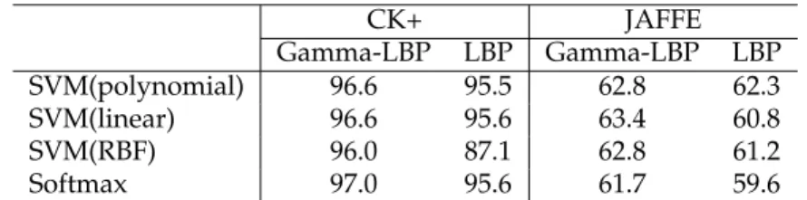
Table 4. Recognition rates on different classifiers with and without gamma correction

CK+ JAFFE

Gamma-LBP LBP Gamma-LBP LBP

SVM(polynomial) 96.6 95.5 62.8 62.3

SVM(linear) 96.6 95.6 63.4 60.8

SVM(RBF) 96.0 87.1 62.8 61.2

Softmax 97.0 95.6 61.7 59.6

Table 5. Recognition rate on CK+ under LBP feature in different literature

Methods Zhong2012[3] Shan2009[4] Proposed Methods

Classifier SVM SVM SVM

Validation Setting 10-Fold 10-Fold 10-Fold

Performance 89.9 95.1 96.6

other methods. The results are shown in Table 3. Several comparison experiments are designed, SVM and classifier is applied to evaluate our algorithm. Comparing LBP features extracted from the alignment areas with the features extracted from salient areas on alignment faces and the whole alignment faces, better recognition rates can be gained by our algorithm by using SVM classifier. Polynomial, Linear, RBF kernel SVM are used in our experiment and the SVM classifier is designed by Chih-Chung Chang and Chih-Jen Lin [29]. Gamma correction method is used to process the LBP features in our experiment. Comparing with the experiment designed by Zhong et al. [3] and Liu et al.[2], according to the results in Table 3, our algorithm has more precise recognition rate.

4.2. Feature Correction and Feature Fusion

In our algorithm, LBP and HOG features are used to train the SVM and softmax classifiers and these features all are extracted from salient areas. In section 2.3, a method has been proposed to process the LBP features and the relationship between theσ and gamma number λalso has been found. In this part, comparing experiments are designed to evaluate the performance of gamma correction. In our experiments, the number of λ is changed from 0.1 to 3 and all these results are recorded. In order to show the relationship between σ, gamma correction number λ and the recognition rate clearly, some figures have been draw to display the trend of recognition rate and σ. In Fig. 9 theσ is the sum of the four salient areas’ σ. In the figure, whileλ equal to 1 there is no gamma correction, and from the figure people can know that the biggest recognition rate and the biggestσvalue result from the value ofλnear to 1.8. Besides, comparison experiments are designed to certificate the universality and performance of gamma correction. Apart from that different classifiers are applied to recognize these expressions and by applying these classifiers, we can say that our LBP correction method can be used to different classifiers. The relationship betweenσ andλ of JAFFE database are shown in Fig. 10. These two figures show that our LBP correction method has fine universality power. In addition, for these is fewer images in JAFFE database, we can see that the curves in Fig. 10 are not smooth enough, but their overall trends also correspond with the relationship in Fig. 10. The performances of these experiments are shown in Table 4 and the table shows that gamma correction has significantly improved the recognition rate. In Table 4, ten-fold cross validation is applied on CK+ database and leave-one-person-out validation method is used on JAFFE database.

In Table 5, our experiment’s performance is compared with some researches which use LBP features to recognize these expressions, and we have the same classifier and validation method with these literature. Comparing with these literature, our experiment has better result and this shows that our salient areas definitude methods and LBP correction method have fine performance. In order to gain a better result, LBP and HOG features are fused in our research. Using only the HOG feature,

0 0.5 1 1.5 2 2.5 3

λ _value

0 0.5 1 1.5 2 2.5

σ

value

a

0 0.5 1 1.5 2 2.5 3

λ _value

20 40 60 80 100

recognition rate

b

SVM(polynomial) SVM(RBF) SVM(Linear) Softmax

14 of 17

0 0.5 1 1.5 2 2.5 3

λ _value 0

0.5 1 1.5 2

σ

value

a

0 0.5 1 1.5 2 2.5 3

λ value 20

30 40 50 60

recognition rate

b

SVM(polynomial) SVM(RBF) SVM(Linear) Softmax

Figure 10. (a) Relationship betweenλ andσ on JAFFE database.(b) Relationship between λand recognition rates from different classifiers on JAFFE database.

0 200 400 600 800 1000

dimension number

0.92 0.93 0.94 0.95 0.96 0.97 0.98 0.99

recognition rate

Figure 11.Relationship between PCA dimension and recognition rate.

Table 6. Recognition rate on CK+

Literature Liu2014[10] Liu2015[2] Jung2015[23] Khorrami2015[11] Proposed Algorithm

Method BDBN AUDN DTAGN Zero-bias

CNN+AD

LBP+ HOG

Validation Setting 10-Fold 10-Fold 10-Fold 10-Fold 10-Fold

Accuracy 96.7 95.785 96.94 98.3 98.3

we gain a 96.7 recognition rate and using the fusion method a better result which is 98.3 has reached on CK+ database. Beseides, a similar result has been gained on JAFFE database.

4.3. PCA Dimension Number and Recognition Rate Comparison

In our algorithm, the full dimension of fusion features is 11636 and it is really a huge number. Besides, huge feature dimension can pull in some noise and lead to overfitting. For the PCA method, if the number of the features’ dimension is bigger than the images’ number the principal component number is 1. In order to gain the most proper number, the number of the dimension is changed from 10 to 1000 and by using this method, the PCA dimension can be chosen according to recognition rate. The relationship between PCA number and recognition rate is displayed in Fig.11. The most proper PCA dimension number is chosen according to the recognition rate and the dimension number of the features put into softmax is 80 on CK+ database.

Until this step, the best recognition rate 98.3 is gained under ten-fold-cross validation method on CK+ database. Comparing with the other method in the literature, a state-of-art result has been gained as far as we known. Our result has been compared with other methods in literature and the results are shown in Table 6. These four experiments all used deep networks while hand-crafted features are used in our algorithm. This explains that our algorithm has fine recognition ability by

Table 7. Recognition rate on JAFFE

Literature Shan2009[4] Happy2015[9] Proposed Algorithm

Proposed Algorithm

Proposed Algorithm

Classifier SVM(RBF) SVM(Linear) SVM(Linear) SVM(Linear) Softmax

Validation Setting 10-Fold 5-Fold 5-Fold 10-Fold 10-Fold

16 of 17

extracting features from the salient areas, correcting LBP features and fusing these features. In order to evaluate the adaptability of our algorithm, our algorithm also is applied on JAFFE database. The results from other literature and our algorithm are shown in Table 7. The experiment shows that our algorithm has quite a good adaptability.

5. Conclusion

The main contributions of this paper are summarized as follows:(1) A salient areas definitude method is proposed and the salient areas compared to their neutral faces are found. (2) The idea of normalizing the salient areas to align the specific areas which express the different expressions is firstly proposed. This makes the salient areas found from different subjects have the same size. (3) Features correction method is firstly applied in and this significantly improves the recognition result in our algorithm frameworks.(4) Fusion features are used in our framework and by normalizing these features to the same scale, this significantly improves our recognition rate. By applying our algorithm framework, a state-of-the-art performance on CK+ database under 10-fold validation method using hand-crafted features has been gained. Besides, a decent result on JAFFE database has been obtained too.

In the future, video data processing will be the focus of our research work and we will try to recognize facial expressions from real time videos.

Acknowledgments: This work was supported in part by the National High Technology Research and Development Program 863, China (2015AA042307), Shandong Province Science and Technology Major Projects, China (2015ZDXX0801A02).

References

Bibliography

1. Izard, C.E. The face of emotion.1971.

2. Liu, M.; Li, S.; Shan, S.; Chen, X. Au-inspired deep networks for facial expression feature learning. Neurocomputing2015,159, 126–136.

3. Zhong, L.; Liu, Q.; Yang, P.; Liu, B.; Huang, J.; Metaxas, D.N. Learning active facial patches for expression analysis. IEEE Conference on Computer Vision and Pattern Recognition (CVPR), 2012, pp. 2562–2569. 4. Shan, C.; Gong, S.; McOwan, P.W. Facial expression recognition based on local binary patterns: A

comprehensive study.Image and Vision Computing2009,27, 803–816.

5. Lucey, P.; Cohn, J.F.; Kanade, T.; Saragih, J.; Ambadar, Z.; Matthews, I. The extended cohn-kanade dataset (ck+): A complete dataset for action unit and emotion-specified expression. IEEE Computer Society Conference on Computer Vision and Pattern Recognition Workshops (CVPRW), 2010, pp. 94–101. 6. Jung, H.; Lee, S.; Park, S.; Lee, I.; Ahn, C.; Kim, J. Deep Temporal Appearance-Geometry Network for

Facial Expression Recognition. arXiv preprint arXiv:1503.015322015.

7. Zavaschi, T.H.; Britto, A.S.; Oliveira, L.E.; Koerich, A.L. Fusion of feature sets and classifiers for facial expression recognition.Expert Systems with Applications2013,40, 646–655.

8. Hu, Y.; Zeng, Z.; Yin, L.; Wei, X.; Zhou, X.; Huang, T.S. Multi-view facial expression recognition. IEEE International Conference on Automatic Face and Gesture Recognition, 2008, pp. 1–6.

9. Happy, S.; Routray, A. Robust facial expression classification using shape and appearance features. Eighth International Conference on Advances in Pattern Recognition (ICAPR), 2015, pp. 1–5.

10. Liu, P.; Han, S.; Meng, Z.; Tong, Y. Facial expression recognition via a boosted deep belief network. Proceedings of the IEEE Conference on Computer Vision and Pattern Recognition, 2014, pp. 1805–1812. 11. Khorrami, P.; Paine, T.; Huang, T. Do Deep Neural Networks Learn Facial Action Units When Doing

Expression Recognition? Proceedings of the IEEE International Conference on Computer Vision Workshops, 2015, pp. 19–27.

12. Tian, Y.l. Evaluation of face resolution for expression analysis. Conference on Computer Vision and Pattern Recognition Workshop, 2004, pp. 82–82.

13. Tzimiropoulos, G.; Pantic, M. Optimization problems for fast aam fitting in-the-wild. Proceedings of the IEEE international conference on computer vision, 2013, pp. 593–600.

14. Zhu, X.; Ramanan, D. Face detection, pose estimation, and landmark localization in the wild. IEEE Conference on Computer Vision and Pattern Recognition (CVPR), 2012, pp. 2879–2886.

15. Lee Rodgers, J.; Nicewander, W.A. Thirteen ways to look at the correlation coefficient. The American Statistician1988,42, 59–66.

16. Tariq, U.; Lin, K.H.; Li, Z.; Zhou, X.; Wang, Z.; Le, V.; Huang, T.S.; Lv, X.; Han, T.X. Emotion recognition from an ensemble of features. IEEE International Conference on Automatic Face & Gesture Recognition and Workshops (FG 2011), 2011, pp. 872–877.

17. Evgeniou, A.; Pontil, M. Multi-task feature learning. Advances in neural information processing systems 2007,19, 41.

18. Ojala, T.; Pietikainen, M.; Harwood, D. Performance evaluation of texture measures with classification based on Kullback discrimination of distributions. Proc. 12th IAPR Int. Conf. Pattern Recognit. Conf. A: Comput. Vis. Image Process, 1994, Vol. 1, pp. 582–585.

19. Ojala, T.; Pietikäinen, M.; Harwood, D. A comparative study of texture measures with classification based on featured distributions. Pattern recognition1996,29, 51–59.

20. Heikkila, M.; Pietikainen, M. A texture-based method for modeling the background and detecting moving objects.IEEE transactions on pattern analysis and machine intelligence2006,28, 657–662.

21. Wikipedia. Histogram of oriented gradients. https://en.wikipedia.org/wiki/Histogram_of_oriented_ gradients.

22. Dalal, N.; Triggs, B. Histograms of oriented gradients for human detection. IEEE Computer Society Conference on Computer Vision and Pattern Recognition, 2005, Vol. 1, pp. 886–893.

23. Zhang, W.; Zhang, Y.; Ma, L.; Guan, J.; Gong, S. Multimodal learning for facial expression recognition. Pattern Recognition2015,48, 3191–3202.

24. Person, K. On Lines and Planes of Closest Fit to System of Points in Space. Philiosophical Magazine, 2, 559-572, 1901.

25. Hotelling, H. Analysis of a complex of statistical variables into principal components.Journal of educational psychology1933,24, 417.

26. Kanade, T.; Cohn, J.F.; Tian, Y. Comprehensive database for facial expression analysis. Fourth IEEE International Conference on Automatic Face and Gesture Recognition, 2000, pp. 46–53.

27. Lyons, M.; Akamatsu, S.; Kamachi, M.; Gyoba, J. Coding facial expressions with gabor wavelets. Third IEEE International Conference on Automatic Face and Gesture Recognition, 1998, pp. 200–205.

28. Lyons, M.J.; Budynek, J.; Akamatsu, S. Automatic classification of single facial images. IEEE Transactions on Pattern Analysis & Machine Intelligence1999, pp. 1357–1362.

29. Zheng, Y.; Capra, L.; Wolfson, O.; Yang, H. ACM Transactions on Intelligent Systems and Technology-Special Section on Urban Computing. ACM Transactions on Intelligent Systems and Technology 2014,5.

c