Computer Simulation and Energy-Saving
Analysis of a Composite Steel Residential
Building
XiaoTong PengUniversity of Jinan, Jinan, 250022, China Email: [email protected]
Chen Lin
Shandong University of Art & Design, Jinan, 250011, China Email: [email protected]
Abstract—The steel frame-reinforced concrete core wall structure is a typical composite structure, which has been applied to residential buildings for its excellent seismic behavior. In order to evaluate the energy consumption of existing residential buildings with composite structures, an on-site test on envelope of a typical composite steel residential building in cold region is performed; the heat transfer coefficient K of envelope and its actual energy consumption are calculated and analyzed by use of the testing data. Based on that, a simplified computer model is established and verified. Parameter analyses are carried out on two main influential factors. The results indicate that the building envelope has good heat storage property and it could keep indoor thermal stability; the steel frames and windows have heat bridge effects;the tested building only meet requirements of energy-saving 50%-standard, instead of 65%-standard; the traditional calculation method for energy consumption overestimates the energy consumption of buildings; the most effective way to reduce heating consumption is to improve thermal performances of external walls; the thickness of insulation layers should be confined in an appropriate range. Finally the thermal design recommendations for composite steel residential buildings are proposed.
Index Terms—computer simulation; energy conservation; thermal insulation; residential building; test; energy consumption; building envelopes
I. INTRODUCTION
Steel structures have become the most popular structural forms of tall buildings for its lightweight, good ductility and seismic performance. It also improves the safety and reliability of residential buildings. Previous studies on the safety of steel structures focused on the dynamic characteristics under seismic load, connection performance, and fire-resistant property and design [1-2], in which the energy dissipation of steel structures was not
involved. The study on the energy saving of steel residential buildings was limited to warm winter and cool summer regions [3-4], while in cold area it was not concerned. Field (on-site) tests of energy saving on steel structures are required to collect energy dissipation data, generalize energy dissipation property and evaluate if envelope details could satisfy requirements of the Design Standard of Energy-saving by 65% for Residential Buildings [5]. In this paper, field test for energy saving is performed using the heat flow meter method by taking a typical composite steel residential building in Shandong province of china as an example. Through calculating and analyzing the test data, the heat insulation and energy saving properties of building envelopes are evaluated, the energy dissipation characteristics of steel residential buildings are summarized, A computer analytical model is established to simulate the energy consumption of the building by use of the software DeST-h, which is a FEM software that mainly focuses on dynamic energy consumption of buildings. Through comparison to the test results, the computer model is verified. Based on that, Parameter analyses are carried to evaluate the energy consumption of buildings. Finally, design recommendations on energy-saving are proposed.
II.ON-SITE TESTS
A. Project Outline
A typical dwelling house, named the Eiffel Garden, is test based on the extensive investigation of existing steel residential buildings in Jinan city of Shandong province The Eiffel Garden, which has 11 floors above the ground and 1 floor under the ground, is designed and constructed according to the Standard for Energy-saving Performance of Civil Construction (JGJ26-95). The heat insulation composite wallboards with 130mm in thickness and the cast-in-site reinforced concrete roof plates were used; haydite concrete hollow blocks with 200mm thick were used as walls around households, staircases and basements, and were built up to the underside of floor plates.
Manuscript received Dec. 1, 2010; revised Jan. 5, 2011; accepted Jan. 12, 2011.
B. Testing Procedures
The heat flow meter method was used in the field testing of the steel residential building envelope. Heat transfer coefficients were evaluated according to the testing temperatures of inside and outside surface and heat flow values. Based on limits of heat transfer coefficient specified in the code, the tested envelope was estimated whether it could satisfy the requirement of energy saving buildings. The procedure was described as follows:
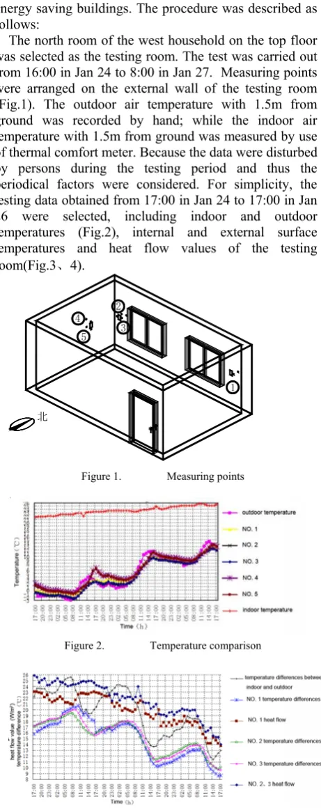
The north room of the west household on the top floor was selected as the testing room. The test was carried out from 16:00 in Jan 24 to 8:00 in Jan 27. Measuring points were arranged on the external wall of the testing room (Fig.1). The outdoor air temperature with 1.5m from ground was recorded by hand; while the indoor air temperature with 1.5m from ground was measured by use of thermal comfort meter. Because the data were disturbed by persons during the testing period and thus the periodical factors were considered. For simplicity, the testing data obtained from 17:00 in Jan 24 to 17:00 in Jan 26 were selected, including indoor and outdoor temperatures (Fig.2), internal and external surface temperatures and heat flow values of the testing room(Fig.3、4).
4 3 2
1 5
北
Figure 1. Measuring points
Figure 2. Temperature comparison
Figure 3. Temperature difference of walls
Figure 4. Temperature difference of roofs
III. TESTING RESULTS AND ANALYSIS
As shown in Fig.2, the outdoor temperature had a great increase about 10°C. The indoor temperature remained between 22°C to 24°C, demonstrating the good heat insulation performance of building envelope. The surface temperature of the external wall had the same variation as the outdoor temperature. From 17:00 to 7:00 at night, the temperature values of outside surface of the external wall were higher than those of the outdoor temperature, so that the heat was transferred to the outdoor air through the wall. The outdoor temperature increased in the daytime because of the solar radiation, so that from 11:00 to 16:00 the temperature values of outside surface were lower than those of the outdoor temperature, and the wall got heat from outside. The wave crest and trough of the outside surface temperature curve lagged behind the outdoor temperature curve’s, showing that the heat insulation property had a delay effect on the temperature wave.
The phenomenon of heat bridges appeared at the steel columns, external windows and room corners. As shown in Fig.3, the heat flow values were proportional to the temperature differences between external and internal surfaces. The heat flow and the temperature differences of No.2 and 3 test points on the north wall near the steel column were bigger than those of No.1 test point far from the steel column respectively. It showed that the closer to the heat bridge the more heat will dissipate.
As shown in Fig.4, the temperature differences between the external and internal surface of No.4 and No.5 test points had a 24-hour periodic variation, that is, the temperature differences started to increase at 17:00, and reached the maximum at about 6:00 on the next day then decreased to the minimum at 17:00, whereas the heat flow took on linear decrease. Therefore, the solar radiation had a great effect on the temperature difference, but the heat flow still remained relative stability because of the heat storage and release property of walls, even though the heat flow decreased under the influence of the temperature difference.
Differences between the value Kp1 and Kp2 of No.2 and 3 test points on the north wall were bigger than those of No.1 test point far from the steel column; the differences between the values Kp1 and Kp2 of No.4 test point on the west wall were bigger than those of No.5 test point far from the steel beam (table 1). Consequently, the closer to the heat bridge the bigger testing heat transfer coefficient will get.
In order to study the effect of Heat Bridge on external walls quantitatively, the testing value KP2 and the average value Km were analyzed as follows.
Km represents the average heat transfer coefficient when the effect of the heat bridge around the perimeter of external walls is considered; it was evaluated by Eq.1 and results were shown in table 2.
2 1
2 2 1 1
B B p
B B B B p p m
F F F
F K F K F K K
+ +
⋅ + ⋅ + ⋅ =
. (1)
Where, FP—areas of the main part of external walls, m2; Kp—heat transfer coefficients of the main part of external walls, w/ (m2·k);
FB1、FB2—areas of the heat bridge around the perimeters of external walls, m2;
KB1、KB2—heat transfer coefficients of the heat bridge around the perimeter of external walls, w/(m2·k).
As presented in Table2, when heat bridges were considered, the values of Km were bigger than the testing heat transfer coefficients Kp2; the area of west wall was smaller than that of north wall, and the heat bridge on west wall took bigger area than on the north wall, so that the heat bridge had significant effects on the heat transfer coefficient of west wall. The heat transfer coefficients could affect heat transfer coefficients by 10%-15%. Therefore, the average heat transfer coefficient Km would reflect heat transferring situation more accurate than Kp2.
Through comparison, the testing heat transfer
coefficient Kp2 of the main part of external walls did not satisfy the requirement of energy saving by 50%. When heat bridges were considered, the value of Km further increased, showing that the heat bridge weakened the thermal performance of external walls. The theoretical heat transfer coefficients of the roof and partitions satisfied the limits of 65%. The heat transfer coefficient of windows only met the requirement of the energy saving by 50%. The shape coefficient of buildings and the window-wall ratio met the requirement of energy saving by 65%.
IV. COMPUTER SIMULATION AND ANALYSIS
A. Simulation Procedure
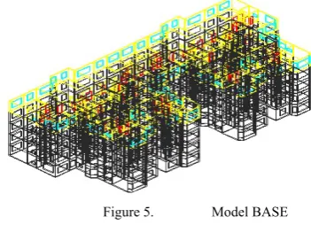
A computer model was established by using the general software DEST-h which is designed to analyze the thermal performance of buildings. In order to save the computing times, the model was simplified as follows: the stories that had same thermal conditions were merged and then the model was simplified into a model with 5 stories (Fig.5). The simplified model was validated by compared to a model with 11 stories and a model with 26 stories (prototype). The comparison results show that from the model with 5 stories to the model with 26 stories, the energy consumption for heating are 13.85w/m2, 13.65w/m2 and 13.54w/m2 respectively, and the maximum calculation error is only 2.2%. It indicates that the simplified model with 5 stories could represent the prototype model with 26 stories.
Figure 5. Model BASE
The parameters in the model, such as building orientation, figure coefficient, window-wall ratio and layout, is consistent with that in prototype building. The heat transfer coefficient, indoor thermal disturbance (Table 3) and outdoor hourly dry bulb temperature in the model were adopted from on-the-spot survey.
TABLE 1 HEAT TRANSFER COEFFICIENT K(w/m2⋅k)
Measuring Points Northern wall Western wall No.1 No.2 No.3 No.4 No.5
Theretical values (Kp1) 0.948
Testing values (Kp2) 1.052 1.059 1.055 0.908 0.895
Mean Value of Kp2 1.055 0.902
Difference of Kp1 and
Kp2(%) 9.8 10.5 10.1 -4.4 -5.9
TABLE 2 COMPARISON OF KM AND KP2(w/m2⋅k)
Measuring Points No.1、2、3 No.4、5
Mean Value of Kp2 1.055 0.902
Mean Value of Km 1.159 1.063
Difference of Km and Kp2(%) 9.0 15.1
TABLE 3 INDOOR THERMAL DISTURBANCE
Position Living Room
Main Bedroom
Secondary Bedroom (Kitchen, Toilet)
Occupant Density 3 2 1 Heat Output Per Capita 53w 53w 53w
Light Disturbance 6w/m2 4.3w/m2 4.3w/m2
B. Model validation
Based on the model described above, the calculated hourly indoor temperature was compared to that from on-the-spot survey (Fig.6). Only the testing data from Jan 22 6:00 am to Jan 23 6:00 were listed in figure 6 for limited print pages. It can be seen that the two curves tally closely and error is less than 5%. The calculated values are bigger than testing values in daytime and smaller in the night for the reasons that ceilings and walls are made from inert materials which have thermal properties: heat storage and release. Those thermal properties could not be simulated by DEST-h. In general, the calculated values match well with tested values showing the DEST-h model is feasible.
Figure 6. Comparison Of Simulated Values And Tested Values
C. Energy simulation
In the specification “energy-saving standards for residential buildings”, the heat transfer coefficient is recommended to evaluate the heat consumption of buildings. The Mathematical model is based on steady heat transfer theory, in which the heat consumption includes three parts: heat transfer quantity of enclosure structures (qH·T), heat consumption quantity of Air Infiltration (qINF) and internal heat gains (qI·H). The calculation formula is qH = qH·T + qINF -qI·H, where qH·T and qINF are calculated on static theories and the indoor and outdoor temperature difference adopts empirical values that are different from the actual values based on dynamic theories. The software DeST is established on dynamic heat transfer theories, and its meteorological Parameters come from typical meteorological year data base. In the simulation procedure, the heating and air conditioning system is used instead of central heating system to calculate heat consumption for DeST’ deficiencies. The concrete method is described as follows: the control temperature of air conditioning system is 20.5 according to mean values of measured indoor temperature, and the air conditioning is open all the day. As shown in the table 4, the traditional calculation values are bigger than DeST simulation values about 5.7%, which is reasoned that the traditional calculation method has not considered solar radiations and neglected the indoor thermal disturbance, thus resulting in errors between traditional calculation values and simulation values. The traditional calculation method overestimates energy consumption of buildings, and measures need be taken to improve the method.
D. Parameter analysis
Through tentative calculations, there were two main factors that affect the energy consumption of buildings significantly. They are insulating layer of exterior walls and roofs. In order to study effects of the two factors on energy consumption quantitatively, two series: WT (wall insulating layer thickness) and RT (roof insulating layer thickness) sum up to 11 models were established, in which the thermal insulating material used plastic benzoic boards (XPS) for its popularity. The prototype model was designated as model BASE. Parameter setting of the two series and energy consumption results are listed in table 5.
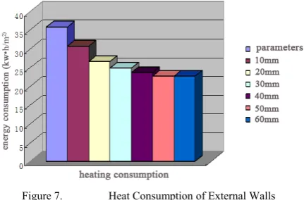
Increasing the thickness of insulating layers of exterior walls (WT) would decrease heat energy consumption greatly. When WT increased from 0mm to 60mm, the heat energy consumption dropped 36.70 %( Fig.7). it is reasoned that in cold region, differences in temperature between indoor and outdoor are greatest in winter, and the differences enhance the heat current effects. The thicker insulating materials could decrease heat currents from indoor to outdoor leading to drops in the heat energy consumption.
Figure 7. Heat Consumption of External Walls
The top floor consumed heat energy most in the building. As shown in the Fig.8, increasing insulating materials improve energy consumption of the top floor significantly than the whole building. From whole building perspectives, when the floor thermal insulation boards increased to 70mm in thickness, the energy consumption decreased only 4.05 KW·h/m2; from the top floor perspectives, when the floor thermal insulation boards increased to 70mm in thickness, the energy consumption decreased 18.53KW • h/m2, and the decreasing range reached 28%. Thus improving thermal performance roof would decrease the energy consumption of the top floor significantly, but has only a little effect on energy consumption of the whole building.
TABLE 4ENERGY CONSUMPTION COMPARISON
Heat Consumption(w/m2)
Error(% ) Traditional calculation
value
Simulation value (DeST-h)
Figure 8. Heat Consumption of Roofs
V. CONCLUSION
The typical residential building only meets requirements of energy-saving 50%-standard, instead of 65%-standard; the external walls and windows are main energy dissipation parts that responsible for 80% of the total energy consumption; the energy consumption of household doors is relatively small, but its consumption per unit area is big, so that the heat insulation property of household doors should be improved if conditions allow; the roof, floor and partitions of staircases have relatively small energy consumption so that the original scheme is still suitable to them.
The heat flux of building envelopes is proportional to the temperature difference between external and internal surfaces, that is, the bigger temperature difference is, and the bigger value of heat flux will be. The heat flux on external walls distributes unevenly; the closer to the heat bridge the bigger value of heat flux will get, and more heat will dissipate. The temperature variation on the external surface of external walls lags behind the outdoor temperature variation, indicating that the heat insulation performance of external walls has delayed effects on the temperature wave. Under the solar radiation, the temperature of external and internal surfaces changes periodically; however, due to the storage and release property of walls, the heat flux still remains relative stability even though it decrease with the variation of temperature difference.
When the heat bridge is considered, the average heat transfer coefficient KM of external walls increases approximately by 15% than the heat transfer coefficient
KP of the main wall, revealing that the thermal performance of the whole walls would be weakened because of heat bridges, therefore, the value of KM is suitable for evaluating the thermal performance of walls with heat bridges.
The traditional calculating methods for building energy consumption existed defects, by which the calculating results is larger than the actual energy consumption. The new calculation method introduced in the paper, in which dynamic energy consumption theory, solar radiation and indoor thermal disturbance are considered, could obtain the more real energy consumption values.
Improving thermal performances of the building enclosure structure would decreases heat consumption effectively. External walls are main parts of enclosure structure, so the best and effective way is to make saving modification for external walls. As far as energy-saving is concerned, the thickness of insulating layer should vary in a specific range. Once the range is exceeded, increasing thickness of insulating layer has no meaning. Comprehensively considering the economy and energy-saving effects, the thickness of insulating boards for external walls (XPS) is 40mm.
The Top floor consumed much more energy than other floors in buildings. Improving roof insulating properties would increase energy-saving performance of the top floor significantly but has a little effect on energy-saving performance of the whole building.
ACKNOWLEDGMENT
The work was supported by the science and technology key projects of Shandong province under Grant No. 2008GG10007002.
REFERENCES
[1] Li Guoqiang, Zhou Xiangming and Ding Xiang, “Shaking
table study on a model of steel-concrete hybrid structure tall buildings,” Journal of Building Structures. Vol. 22, 2001, pp. 2-7 (in chinese).
[2] Peng Xiaotong, Gu Qiang and Lin Chen, “Experimental
study on the steel frame-reinforced concrete infill wall structure with semi-rigid joints,” China Civil Engineering Journal. Vol. 41, 2008, pp. 64-69 (in chinese).
[3] Wang Rui, “Discussions on measuring methods of energy saving assessment of residential building in cold winter and hot summer area,”New Building Materials. Vol. 10, 2007, pp. 57-59 (in chinese).
TABLE 5 PARAMETER ANALYSIS
WT Series
Thickness (XPS)mm
Heat Transfer Coefficient
[w/(m2·k)]
Energy
Consumption RT Series
Thickness (XPS)mm
Heat Transfer Coefficient
Energy Consumption (Top Floor)kw•h/m²
WT1 10 0.7 30.7 RT1 15 0.62 34.10(58.49)
WT2 20 0.577 26.59 RT2 25 0.513 33.65(55.30)
WT3 30 0.502 24.9 RT3 40 0.406 33.04(51.90)
WT4 40 0.427 23.7 RT4 55 0.34 32.16(49.72)
WT5 50 0.378 22.78 RT5 70 0.29 31.82(48.10)
WT6 60 0.339 22.69 BASE 0 0.899 35.87(66.67)
[4] Dong Mengneng, Lv Zhong, Mo Tianzhu, “Quantitative Analysis on the Effect of Thermal Bridges on Energy Consumption of Residential Buildings in Hot Summer and Cold Winter Region,” Journal of Chongqing Jianzhu University. Vol. 30, 2008, pp. 5-8 (in chinese).
[5] DBJ 112602—2006,Specification for Energy Saving of Residential Buildings (in chinese) .
[6] Li Zheng-Rong, Zhang Hai-Dong, Tang Ze, et al.
“Research on the influence of external window on energy consumption of residential building in the hot summer and cold winter zone.” Journal of Harbin Institute of Technology (New Series), Vol. 14, 2007, pp. 34-37.
[7] Swan Lukas G, Ugursal V Ismet. “Modeling of end-use
energy consumption in the residential sector: A review of modeling techniques,” Renewable and Sustainable Energy Reviews, Vol. 13, 2009, pp. 1819-1835.
[8] Kauhala Kari. “Simple computer model for estimating the energy consumption of residential buildings in different microclimatic conditions in cold regions,” Energy and Buildings, Vol. 16, 1991, pp.561-569.
[9] Wong L T, Mui K W, Law L Y. “An energy consumption
benchmarking system for residential buildings in Hong Kong,” Building Services Engineering Research and Technology, Vol.30, 2009, pp. 135-142.
[10]Michopoulos A, Martinopoulos G, Papakostas K, et al. “Energy consumption of a residential building: Comparison of conventional and RES-based systems,” International Journal of Sustainable Energy, Vol. 28, 2009, pp.19-27.
[11]Chen Shu-Qin, Yoshino Hiroshi, Li Nian-Ping. “Statistical analyses on summer energy consumption characteristics of residential buildings in some cities of China,” Energy and Buildings, Vol. 42, 2010, pp. 136-146.
[12]Yang Yu-Lan, Li Bai-Zhan, Yao Run-Ming, Et Al. “A
method for energy efficient assessment and labeling of residential buildings,” Journal of Civil Architectural & Environmental Engineering, Vol. 32, 2010, pp. 105-112.
[13]H Yoshino, J C Xie, T Mitamura. “A two year
measurement of energy consumption and indoor temperature of 13 houses in a cold climatic region of
Japan,” Journal of Asian Architecture and Building Engineering, Vol. 5, 2006, pp. 361-368.
[14]Fukushima I, Urano Y, Watanaba T. “Study of housing
energy consumption in the Kyushu area,” Journal of Society of Heating Air-conditioning and Sanitary Engineers of Japan. Vol. 57, 1995, pp. 35-48.
[15]Jian Yi-Wen. “Validation study of simulation software of dest,” Journal of Beijing University Of Technology, Vol. 33, 2007, pp. 46-50.
Xiaotong Peng ShanDong Province,
China. Birthdate: Oct, 1973. is a Civil Engineering Ph.D., graduated from Dept. Civil Engineering Xi’an University of Architecture and Technology. And research interests on seismic behavior and energy-saving of composite steel structure. He is an associate professor of school of civil engineering and architecture, University of Jinan.
Chen Lin ShanDong Province, China.
Birthdate: Jul, 1977. has Architectural Technology Science Master Degree., graduated from Dept. Architecture Xi’an University of Architecture and Technology. And research interests on energy-saving of buildings.